A Random Multi-Trajectory Generation Method for Online Emergency Threat Management (Analysis and Application in Path Planning Algorithm)

Robot path planning have been witnessed a great achievement these years with the various application of robots. Problems such as path planning, motion planning, and online moving obstacle management have been widely studied toward the goal of performing autonomy. Unmanned Aerial Vehicles (UAVs), an easy access robot platform, has been increasingly applied in research and commercial areas in recent years. UAV autonomy denotes the ability of tackling with obstacle (or called no-fly zone) avoidance and trajectory planning online from a starting position to a destination while satisfying the kinematic constraints.

For robot path planning, emergency threat management (ETM) is one of the hardest challenges that needs to be solved, where a sudden threat may burst into view or dynamic obstacles are detected on line, especially when UAV is following the desired path. Under such conditions, UAV should consider the following attributes:

1. Time efficiency: The most important requirement for ETM algorithm is time efficiency. For general ETM, the configuration is periodically updated, such as heuristic algorithm A*, which it is computationally intensive if the map is represented with high resolution. In order to guarantee safety, ETM requires real-time performance.

2. Kinematic feasibility: Kinematic feasibility denotes that the output of the planner meets the kinematic constraints of the robot as well as the environment. The constraints include: (a) Path smoothness: The planner is required to output kinematic smooth path, sometimes even kinodynamically feasible as well. Thus, the path should meet the state of art tracking constraints, and enables low tracking error for UAV; (b) Minimum cost of switching: The strategy of handling the threat, especially ET, is to find the cost minimum path by generating a new path or multiple paths besides the initial one. The cost for choosing the best path should take the dynamic constraints, energy consumption and time performance into consideration.

3. Specific requirements: UAVs have already been applied to many areas, such as inspection, photography, and monitoring. They have to meet some specific requirements according to environments and system constraints. For example, best pose based illumination of tunnel inspection for crack and spalling, and stable tracking with obstacle avoidance as UAV photography which should be able to keep stable capturing even during the flying.

Development with open robot platform and field implementation has witnessed the promising performance of Sampling Based (SB) methods. SB algorithms (SBA) have the advantages for planning in high dimensional space, and it is with the ability to deal with multiple classes of path or motion planning problem in both static and dynamic environment. Rapidly-exploring random trees (RRTs) are single query methods which obtain Voronoi biased property and only generate homotopy paths simultaneously. Although it proposes to solve the multiple degrees of freedom (DOF) operating problems in known static environments, SBA shows great performance of dealing with any kind of path or motion planning problem in complex environments for unmanned ground robots or aerial robots.

In this paper, we introduce two biased-sampling methods, which are obstacle biased and Homologous Classes (HC) biased to perform path planning respectively. For obstacle biased path method, we have discussed in with UAV demonstration. For HC classed biased approach, it aims at solving the ET problem by generating alternative paths for online dynamically switching. HC introduces an online dynamic reconfiguration approach to ensure singularity between paths, which tries to generate more paths with different obstacle reference. Thus, it can perform alternative switching online when confronted with ET. The obstacle biased planning method is called Guiding Attraction based Random Tree (GART) and HC biased is called Multi-GART (MGART). We consider the environment to be known as a priori to us, and the UAVs are with the ability to understand the clearance region. Experiments and comparative simulations are illustrated to provide the effective evaluation of the proposed methods.

Preliminary materials

HOMOLOGY AND HOMOTOPY

For path planner, the purpose is to find a feasible path p_f (cost minimum or complete) from the initial position to the goal position in the workspace W ∈ R^{n}, n denotes the dimension of space the robots locate. A general cost function can be represented as:

The cenergy,ctime,cthreat cost, time consumption, and threat respectively. These costs are not fixed, since the energy cost can be path length, and time consumption can change according to the velocity limitation. For cost constrained path planner, the goal is to find the asymptotic optimal rather than the completeness solution. Then, more than one path can be found during the process, and the paths can be homotopic or belong to different homotopic classes (or called homology).

It is illustrated in Figure 1. Given a continuous map H : I × I → Γ or H : h(s, t) = h_t(s), Γ denotes the topological space and I = [0, 1] is the unit interval. The obstacle regions are labeled with R_o1, xinitial=h(0,t)denotes start point, xinter=h(1,t) denotes the goal position, x_inter denotes an inter node for obstacle avoidance. For the continuous deformation, given h(s, 0) = π₀, h(s, 1) = π₁, the path can be continuously mapping through π₀ to π₁ with t ∈ [0, 1]. For any path deformed between, they are homotopic with π₀, π₁ if and only if they stay in the closed loop π₀ ∐  − π₁, where the closed loop cannot collide with any obstacle region.

Definition 1—Homotopic Paths: It denotes the equivalence class of all paths under continuous mapping H : h(s, t) = h_t(s), which locates in the closed loop formed h(s, 0) ∐  − h(s, 1). Any path in the set can be continuously deformed into any other without colliding with any obstacle in the space. For all paths in the set, they are with the same fixed end points.

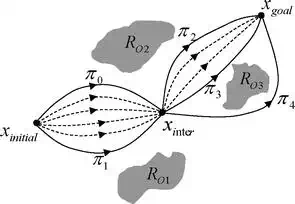
FIGURE 1.

Homotopic and homologous classes and paths.

We can conclude that π₂ and π₃ belong to the same homotopic class. However, we can find path π₄, which shares the same start and ending node, cannot be continuously deformed to π₃ due to the isolation of the obstacle. It means (π₃ ∪  − π₄) ∩ R_o3 ≠ Θ. In such case, we call π₃ and π₄ are homologous, and they belong to different homotopic classes.

Definition 2—Homologous Paths: Paths, which follows the same continuous mapping H : h(s, t) = h_t(s), cannot form a closed loop by h(s, 0) ∐  − h(s, 1). The homologous paths belong to different homotopic classes.

PROBLEM STATEMENT

Path planning follows a common procedure to perform trial and error process under empirical constraint to achieve completeness. The problem of path planning does not only solve a problem for exploration optimization, but also try to model the environment with a best descriptor as discussed in. Let us take a look again with the problem of path planning which can be represented as:

The path h(s) (homologous) should stay in obstacle free region R_free, that is, h(s) ∈ R_free. Usually, the path is piecewise continuously, and it can also be smoothed to obtain first order continuous thus to ensure kinematics continuous. Besides the exploration to achieve completeness (in Eq. (1)), the obstacle modeling method is also important and affect the planning results.

To solve this problem, this paper proposed a multi-path online switching approach, that is, the path planner can find alternative homologous-paths. Then, this paper designs an online fast switching strategy. For multiple path planner, it aims at finding as many paths as possible,

H_alter denotes the set of all the alternative paths hⁱ(x(t), u(t)), x(t) denotes the state, and u(t) denotes the control. However, the mission planner cannot use all the planed paths for online switching, it should find the reasonable paths without redundancy. We propose the follow rule,

H_reason denotes the paths set where any two paths are not homotopic to each other, H≠ denotes non-homotopy. Now, we have the paths which keep distinguishable from each other with different obstacles sequence surrounding.

Rapidly exploring random tree path planner

In this section, we try to describe the underlying research of rapidly-exploring random tree (RRT, upon which we propose a novel state of art approach to facilitate the active exploration in cluttered environments). SBAs are incremental search algorithms which perform random sampling with collision checking for extension, and they were first proposed to solve high dimension planning problem. They have the merits of considering the control and kinematics constraints together, and can incrementally construct a tree from the start node (or initial state) to the goal node (or goal state) with continuously sampling and expansion.

It is shown Figure 2, the whole tree graph by exploration is represented as G_T, the black solid dot denotes the valid state within step accessibility under kinematics constraints, and the black solid lines connect each parent state with child state for extension. Every step, a new sample g_sample will be generated randomly. It should be cleared to all that the initial random sampling does not mean a fixed connection, that is, the random sampling can be a direction for extending. Then, the random sample g_sample tries to find the nearest state in the tree for connection under minimum Euclidean metric,

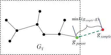
FIGURE 2.

RRTs propagate by applying the minimal cost criterion to connect the newly sampled guard to the previous tree.

Where g_i is an element of all valid states set G_T.

RRT CONNECTION WITH KINEMATIC CONSTRAINTS

For RRT planner, given a system with state (xẋ ,xẏ ,θ̇ )xẋxẏθ̇, and a general form of system model:

It can extend with simply random sampling with control inputs [u_x, u_y, u_θ]. The random sample has to follow the kinematics constraints. Given the robot system, the differential constraints can be represented as a set of implicit equations as g(x,ẋ )=0gxẋ=0, and it can be further represented as:

Here, x denotes the state, and u ∈ U denotes the valid control in allowable controls set. Given the parent state g_parent(t), the time step follows a Δt limits. Then, the control inputs vary with u = {u(t^′)| t ≤ t^′ ≤ t + Δt}. To compute x(t + Δt), we can follow a typical procedure as [12]. It should be noted that the planner should extend toward the newly sampled g_sample. The planner first computes the possible region of reachability from current state x(t):

where ϵ is the maximum first order factor of control input. RRT now picks a new state along the direction from parent to new sample, that is, g_new ∈ [x(t) + f(x(t), u(t) − Δt ∙ ϵ), x(t) + f(x(t), u(t) + Δt ∙ ϵ)] and g_new = g_parent + δ(g_sample − g_parent) with δ ∈ [0, 1].

VORONOI BIASED INCREMENTAL SEARCH

Before discussing the Voronoi biased property of the SBAs, let first introduce some basic notation. Given a set of points S = {s_i| i = 1, 2, …, n} in a n-dimension space Χ. For any two distinct points s_p and s_q in set S, the dominant region (Voronoi region) of s_p over s_q is defined as the region where any inside point should be closer to s_p over s_q, that is,

Where χ is the dominant region corresponding to s_p, ||^L denotes the Lebesgue measurement. In a normal case, any point s_i has its own dominant region with,

Normally, random sampling of RRT follows a Monte-Carlo Method to perform an uniformly sampling in a n-dimensional space under Lebesgue measurement. We can look back at the beginning of Section 3, the new sampled node tries to connect to the nearest node under Euclidean metric. We can now analyze the problem in another perspective that given g_parent and g_s, they connect to the same origin g_o. Then, a new sample g_sample is generated randomly following a Monte-Carlo process. In order to explore and reach the goal, g_sample tries to connect to the tree following the metric defined in Eq. (5). It means that g_parent and g_s can be connected for expansion under minimum distance principle, then g_sample has to be assigned to the dominant region which subjects to a closer point (the Voronoi region). Under this principle, g_parent and g_s can acquire new resource for extension with the ability to keep distinct region and extending their branches.

A typical Voronoi-biased exploration using sampling can be seen in Figure 3, where each branch keeps distinct with each other to form a star network like structure and it behaves the same for heuristic informed RRT. Here, unlike the dominant region of a point, RRT branch can be also treated as a distinct individual with its own Voronoi region for acquiring the extending resource.

FIGURE 3.

Results of incremental exploration of RRT and hRRT [16] after 200 and 1000 iterations, respectively.

Obstacle and homology biased path planner

In this Section, we propose approaches to solve two main problems, which are handling cluttered environment and online ET processing, using obstacle-biased method and homology-biased method. Collision detection during the incremental exploration is time consuming, and it follows a routine procedure to guarantee safety. It should be noted that the step validation of each new sampling state provides the directional information of obstacle distribution.

OBSTACLE BIASED PATH PLANNER UNDER KINEMATIC CONSTRAINTS

SBAs mostly deploy the general idea of generating random samples for incremental exploration, and the sample locating in obstacle region will be discarded since it is time consuming and no benefits for increasing the performance of exploring. We firstly deployed a simple idea which was proved to have much higher time performance then RRT and RRT* in.

This paper introduces an obstacle biased algorithm, using obstacle information to help generating more samples for connection. It is shown in Figure 4, the newly sampled states xs1,xs1x1s,x1s tries to connect to the nearest state in the tree. However, xs1x1s leads toward the obstacle region, xs2x2s locates in obstacle region. To use the obstacle information, this paper proposes an active exploring method, that is, inner propulsion and outer attraction.

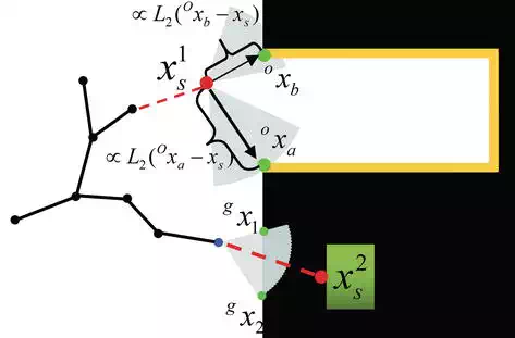
FIGURE 4.

Obstacle biased SBA uses the obstacle location as input, with inner propulsion and outer attraction, to generate more samples for exploration. xs1,xs2x1s,x2s are new samples, the black region denotes obstacle region.

For outer attraction, new sample xs1x1s performs a collision checking, and find the nearest nodes ^ox_a, ^ox_b. We define that the further the obstacle to the sample, the more attraction it can support, that is, the attraction is proportional to the distance between obstacle and the sample using L2-norm L₂. The sample then re-allocation by add a obstacle biased attraction as:

Where k is a constant to adjust the shifting percentage of the attraction vector.

The inner sample in collision with the obstacle is regarded to provide guiding information for the algorithm. This paper tries to find two more states ^gx₁, ^gx₂ within kinematic reachable region (discussed with Eq. (8)), it tries to find out the first two safe state with two directions which are out of obstacle region in the kinematic reachable region (the light blue fan-shaped region). Then, the two newly generated samples ^gx₁, ^gx₂ follows principle Eq. (11) to redistribute to the final position, and connect to the tree.

By using the two proposed approaches, we can generate more useful samples for extending, especially, the samples generate around the edge of the obstacles with the ability to perform more active exploration in cluttered environments. Besides, the outer attraction redistributes the samples toward the narrow corridor between the obstacle, which thus increases the probability of finding safe path through such obstacle crowed region.

HOMOLOGY BIASED

We assume any path h_t(s) generated using SBA is consisted by a set of nodes ht(s)={ht|ht(s′),s′∈[0,1]}, as it is illustrated in Figure 5(a) that exploring tree is consist of the red nodes. Each red node is regarded as distinct with other nodes in the tree, with a distinct dominant region, i.e. Voronoi region. Thus, a path h_t(s), which is consisted a set of states from the initial state to the goal, can be isolated with each other with a distinct region V(b_T) combined by all Voronoi regions of the states.

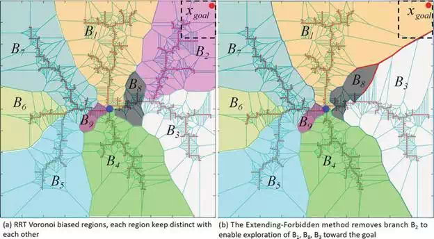
FIGURE 5.

The extending-forbidden algorithm (EFA) tries to find all the states along the goal reached branch at each goal reaching checking step, such as branch B₂. Then, EFA sets the flag of the states to be inactive, switching the extending probability to the nearby branches.

The region dominant property differs the path with each other, where a SB tree with multiple paths (the path here may not connect to the goal, but they keep distinct with each other from the initial position) can be described by a set of branches B_T = {b_T(1), b_T(2), …, b_T(n)}. For each branch, it consists of a list of states which connect with each other to form tree structure. In the tree, the end state relies on the parent state for extending as well as trajectory tracking.

EXTENDING-FORBIDDEN ALGORITHM

The path planner performs exploration following the Monte-Carlo approach. Given a configuration space C in a topological space (the rectangle region as illustrated in Figure 5), we denote the Lebesgue Measurement of the configuration space as L^∗ ∣ C∣. Then we can get the Lebesgue measurement of each branch b_T(i) of the tree using the same metric. Authors in proved that the dispersion of n random nodes sampled uniformly and independently in V(b_T(i)) is,

Where ψ(b_t(i)) denotes the number of samples m, 1 ≤ m ≤ n, that lies in the sub-branch b_T(i), n is the number of all the sampling, d is the dimension of the configuration space. D denotes the difference between the ration of sampling probability and ration of space Lebesgue measurement, which follows the knowledge that Monte-Carlo method performs a uniform sampling. It means the sampling probability approaches the ratio of Lebesgue measurements, that is, the exploration probability can be represented as:

However, the probability of exploring in the configuration space does not benefit the extending bias toward the goal. Let us still take a look at Figure 5(a), the branch B₂ dominant the near-goal region, and other region are not able to extend toward the goal as the samples will not connect to the branches if it locates in the near-goal region. To solve this problem, this paper proposes an Extending-Forbidden Algorithm (EFA), it shifts the source for extending to other branches by forbidding the goal reached path.

Definition 3—Goal-biased Probability: Given a configuration space C, the exploring tree T and all its branches which are main branches B_T and its corresponding sub-branches. The goal-biased event denotes a branch can exploring toward the goal. If a goal region can be represented as G_r, and Voronoi(G_r2B_T(i)) is the region that belongs to goal region and the Voronoi region of branch B_T(i). Then, the nominal goal biased probability of branch B_T(i) toward G_r is:

And the real goal biased probability is normalized value of all branches, that is,

Definition 4—Long Sub-branch (LSB) and Short Sub-branch (SSB): Given a tree T and all its Voronoi distinct main branches B_T. Then, we can define a length threshold δ_B. For all end vertices in each main branch, we calculate the length l_sb from end to the goal reach reached path (any state which firstly reached). If the length l_sb > δ_B, then we call it Long Sub-branch (LSB). If l_sb ≤ δ_B, we call the sub-branch as Short Sub-branch (SSB).

It should be noted that the threshold is very empirical in Definition 4, and it is decided based on the configuration space and the kinematic constraints. In Figure 6, we set it as 15 meters, then we have SSB₁, SSB₂, SSB₃ as SSB, and LSB₁ as LSB. The reason why we have this definition is that we cannot shift all the extending resource to the neighbor branches, and we have the hypothesis that the SSB must has lower probability of finding a new path even given the resource for extending. For example, the main Voronoi dominant branches B_T keep distinct with each other, and each main branch has the probability P_bT(i) for exploration in the configuration space. After the tree stops extending at a certain iteration, we can have the results as illustrated in Figure 5(a). Since goal region is in Voronoi region of branch B₂, then we know that we have the goal biased probability as P_G(B(2)) = 1. One branch B₂reached the goal region which is represented with dotted back rectangle, EFA searches the SSBs and LSBs based on Definition 4, and it labels states and executing forbidden. Then, we have a resource shifted Voronoi graph as illustrated in Figure 5(b), where we can see that branch B₁ and B₃ obtains the Voronoi region which belongs to branch B₂. The two branches also obtain the rectangle goal region, that is, their goal biased probabilities are bigger than zero, P_G(B(1)) > 0, P_G(B(3)) > 0.

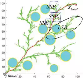
FIGURE 6.

An intuitive example of SSB and LSB in an exploring tree, which are generated using threshold principle as defined in Definition 4.

Since EFA can shift the goal biased by extending resource to other branches, while not all paths can obtain such resource. The following truths are hold:

1. The increasing of goal biased probability ensures the generation of a feasible path toward the goal, but not all branches with goal biased probability can reach the goal at the same time. Only one can reach the goal because of Voronoi dominant probability, thus the general SBA cannot find multiple paths.

2. The efficiency of generating multiple paths mainly depends on the environment adaptability of random exploring algorithms. For random exploring algorithm, their merits of generating multiple branches enable the generation of multiple paths.

REASONABLE ALTERNATIVE REFERENCE CHOSEN

The proposed MGART is able to perform extending-forbidden toward multiple paths, as the random exploring property guarantees completeness and diversity. However, the quality of explored paths cannot be guaranteed, particularly a large number of homotopic paths are generated. This paper proposes an approach to generate the reasonable path, and we analysis under the hypothesis that the environment is highly cluttered and it is not practical to set threshold for path planner to choose the best homological paths.

Definition 5—Reasonable Alternative Paths: Consider two homotopic paths h(π₁) and h(π₂) in a configuration space C. The surrounding obstacle information along each path are ℶ(h(π1)) and ℶ(h(π2)). The reasonable alternative path exists if and only the surrounding information of the two paths are not the same, such that, ℶ(h(π1))≠ℶ(h(π2)).

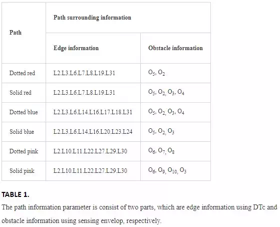
Given the sensing range of a robot as Υ, and the obstacles set O = {o₁, o₂, …., o_n}. For path h(π₁), it consists of a set of discrete states X(π₁) = {x(π₁)₁, x(π₁)₂, …, x(π₁)_n}. In this paper, we assume that any obstacle ο_i can be described with a circle or ellipse centered at ocioic, then we can build a Delaunay Triangulation [19] connection (DTc) using the obstacle centers, the initial state, and the goal state. For DTc, it can generate a network like structure, and each two states have at most one connection. It is illustrated in Figure 8(a) that the green edges are the valid connections, with labels to distinct with each other. For any path, if the path intersects with an edge, the edge information should be added to the information factor, such as the solid red path intersects with edge L7, then L7∈ℶ(h(π1))L7∈ℶhπ1. The edge labeling method can guarantee the uniqueness toward homology, while we note that homotopic paths can also be used to perform emergency threat management. It is represented in Figure 7(b), the solid red path h_s and the dotted red path h_D are homotopic to each other. Given the sensing range Υ, we have the sensing envelop which are dotted purple lines hL1,hR1 for h_D and solid black lines hL2,hR2 for h_s, indicating the maximum detection range for emergency threat. Then, we have the {o1}⊂ℶ(hD) and {o1,o2,o3,o4}⊂ℶ(hS), thus we have h_s and h_D both regarded as reasonable alternative paths for online threat management.

FIGURE 7.

An illustration of surrounding information used to find reasonable alternative path for online emergency threat management. The information parameter consists of edge information and obstacle surrounding information within sensing envelop.

The informative approach discussed thus can help to label each path in a configuration space, such as the results listed in Table 1 of paths in Figure 7(a). Then according to Definition 5, we can find the label of each path. For any several paths which have the same label, we choose the shortest path and use as the candidate for online fast switching.

EMERGENCY THREAT MANAGEMENT

The reasonable alternative path set H_RAP provides a network with cluttered environment adaptivity. The concept of visibility was discussed in, where the cycle information is used to enable fast deformation for motion planning. Visibility is defined as:

Where x₍₎ denotes a state of a path, LlinkLlink is the connection of two states, C_free is the free space and C_obs is the obstacle region. A visual illustration is provided in Figure 8(a), where visibility can only in obstacle free region.

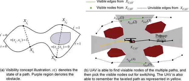
FIGURE 8.

For online switching, UAV should follow the visible-node selection algorithm (a) to explore the possible switching route, then it switches to the cost minimum path for ETM (b).

It is noted that the visibility in this paper means a possible connection to switch from one path to another for emergency threat management. For switching with visibility, given all the reasonable alternative paths H_RAP, the algorithm performs exploration for visibility state at each UAV state x_UAVamong H_RAP. The algorithm then outputs the visible guards (states) x_RAP as illustrated in Figure 8(b). To avoid the pop-up threat (or dynamic threat), UAV must select one entry guard from the visible guard set to reconnect to another pre-planned path to the goal. To validate the best connection, that is, the entry point and the entry connection, this paper applies the heuristic:

Using a simple cost based metric, where C_FE is the forward energy cost which is the distance and the turning cost from UAV position x_UAV to entry state x_RAP(j) and the path from entry state to the goal H_RAP(i)(x_RAP(j)). The turning cost is the integration of heading angle difference at each state, which denotes the smoothness of the planned path. C_TC is the threat cost, the integration of inverse distance between state and obstacles. Using such approach, the algorithm can find five visible states x_RAP = {x_RAP(1), …, x_RAP(5)} as illustrated in Figure 8(b). Then, it tries to find the best entry state using the minimum cost principle (Eq. (17)).

We further consider a situation that there may have no visible states at current location. The paper proposes to use a long-term memory approach to handle this problem, that is, the travel path should be stored in memory, such as the orange edges and states illustrated in Figure 8(b). In the meanwhile, the method stores the visible state along the traveled path. Then, the UAV has to fly back to find a cost minimum path toward the goal if it confronts with pop-threat and has no visible states.

Experiment and discussion

In this section, we highlight the performance of the obstacle biased and homology biased path planner with the ability of emergency threat management (avoiding pop-up and dynamic threat online). In the section, we will discuss the following points: (1) How the threshold of EFA affects the performance of MGART. (2) The time performance and reliability of reasonable alternative chosen algorithm. (3) The online emergency threat management performance. The algorithm is implemented using MatLab 2016b on a laptop computer with a 2.6 GHz Intel Core I5 processor.

COMPARATIVE SIMULATION OF MULTIPLE PATH EXPLORATION

We design three different scenarios, which are non-obstacle scenario, rounded obstacle crowed scenario, and irregular polygons crowed scenario, to perform comparative simulations. All the scenarios are 2D with 100^∗65 m² space, and obstacles randomly generated.

For scenario 1, it is a non-obstacle environment, and we set the variable threshold as a set with value {3, 5, 7, 8, 11,13,15,18,20,25,28} for representation. As we know the length of EFA threshold affects the goal biased probability, which directly decide the area of the newly obtained Voronoi region of the neighbor branches, we design a set of comparative experiments to study the effects between EF length and RAPs. An intuitive result of the relationship between planned paths and EF length after 10,000 iterations are provided in Figure 9(a)–(d). MGART can find 37 paths after 10,000 iterations if EF length is set as 3 step-length, and the number decreases to 22 if the EF length is set as 28. The reason is that the longer the EF length, the further the neighbor branches can obtain the goal biased resource. Thus, the neighbor branches need more steps to exploring toward the goal, that is, less paths will be achieved with better homology performance. As we can see that the paths in Figure 9(d) have a better homology performance than Figure 9(a). The same EF length variation experiment is also deployed in scenario 2, and results are shown in Figure 9(e)–(h). For RAPs, it is the same with the results in scene 1 that RAPs decrease with the increasing of the EF length. However, as the increasing of EF length enables more branches to explore toward the goal as well as increasing the homologous paths (see in Figure 9(e)–(h)), the number of the RAPs increasing with the increasing of the EF length. The statistic relation between the RAPs and the EF length is illustrated in Figure 10, which further proves the conclusion.

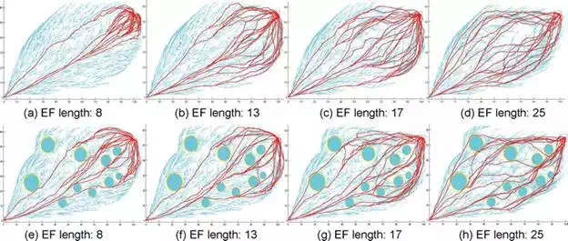
FIGURE 9.

Illustration of alternative paths generated by MGART vary with representative backward EF length. (a)–(d) denotes the results in non-obstacles scenario, (e)–(h) denotes the results in obstacle crowed.

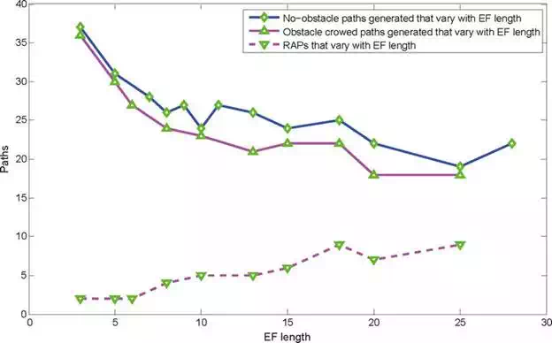
FIGURE 10.

Relation between EF backward length and APs and RAPs with two scenarios. Here the solid diamond line denotes the relation of scene 1, and the triangle lines denotes the results of scene 2.

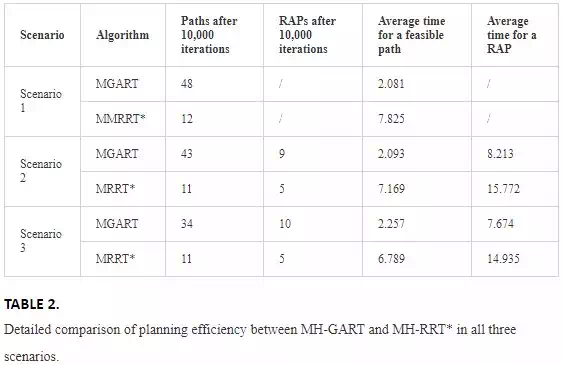
The EFA can be used to any SBAs by shifting the goal biased resource to achieve multiple RAPs for online switching. This paper compares the performance between MGART and MRRT* in three scenarios with 10,000 iterations. We compare the efficiency of generating a path, RAPs, average time for finding a path, and average time for any RAP are compared in Table 2. GART has a better performance in both path exploration and RAP generation, such that MGART can find at least 3 times of the number of paths toward the goal than MRRT*. Because GART introduces the environmental information to speed up the exploring process, the results prove that MGART is more efficient in finding RAPs, which is almost 100% faster than MRRT*. For time performance, we can see that MGART also outperforms MRRT* with at least 3 times advantage.

Besides comparison of the time performance of finding online switching paths (that is RAPs), we also pay attention to the quality of the path generated. The average lengths and standard deviation of the length of all paths in each scene are illustrated in Figure 11. The average length of the paths that generated by MGART and MRRT* are illustrated in Figure 11(a), we can see that MGART has a strong convergence performance than MRRT*. The standard deviation of the lengths is shown in Figure 11(b), results demonstrate that MGART is more likely to find paths with smaller fluctuation as well as smaller cost.

FIGURE 11.

Comparison of (a) average length and (b) standard deviation of the APs generated by MGART and M-RRT* in three scenarios.

PERFORMANCE OF REASONABLE ALTERNATIVE PATH CHOSEN

We also test the path labeling algorithm, that is, the surrounding information pursuing using DTc and sensing envelop, which is used to obtain the reasonable alternative paths under Definition 5. It is should be noted that the under the definition, any two paths do not have the same information parameter, which enables fast switching when facing pop-up threat. As the path label method guarantees the unique labeling of all the paths, only the paths which stretch in a parallel way and within the same sensing envelop have the same labels.

The results of simulation after 10,000 iterations in scenario 2 and 3 are provided in Table 3. For each single path, the time needed for labeling the path mainly depends on the area, dimension, the complexity of the configuration space. For our tested with area 100^∗60, the average time for acquiring the information for labeling 0.078 s (see in Table 3). The average time needs for RAP pursing of our cases is 0.139 s.

Scenario 2		Scenario 3
Time for labeling (s)	Time for RAPs (s)	Time for labeling (s)	Time for RAPs (s)
0.0721	0.146	0.0842	0.132

TABLE 3.

Time performance of proposed method in two scenarios.

EXPERIMENTS OF EMERGENCY THREAT MANAGEMENT

MGART can be used for 3D and 2D pop-up threat management, and the 3D environments can be easily segmented by DT. We evaluate the performance of our method in both 2D and 3D environments, and we also compared the time performance.

For 2D environments, we implement three tests with different number of dynamic threats. The RAP chosen algorithm works when robot realizes that the path will collide with the pop-up threat, that is, robot at position x_UAV detects the moving threat (see in Figure 12(a)). The simulation setting is illustrated in Table 4, where the robot speed is 10 m/s and the moving threat can be detected within 10 m detection range. Thus, the robot has less than 1 s to re-plan a path and executing to avoid the obstacle. RAP chosen algorithm first evaluates all its neighbor RAPs (the green lines) around the robot, and chooses the cost minimal and collision free path based on principle Eq. (17) (the dotted green path in Figure 12(b)). It is noted that Figure 12(b)–(d) are results of using MGART to avoid one, two, and three moving threats, respectively. The black parts along the navigation path denote the position where threat is detected by robot. We also execute test in 3D environment (see in Figure 13) with pup-up and moving threats. The on-line switching is supposed to be used for aerial robots in 3D, thus Dublin’s Curves is used when switching from current position to safe path.

FIGURE 12.

Tests of on-line switching to avoid dynamic threats using MGART in 2D scenarios. (a) Robot detects moving threat at position x_UAV, then it evaluates all its visible neighbor RAPs (the green lines) to choose the switching path. (b) Complete navigation of avoiding one moving threat, the red path is the navigation path. (c) Test of avoiding two moving threats, the black and red circles are threats. (d) Tests of avoiding three moving threats.

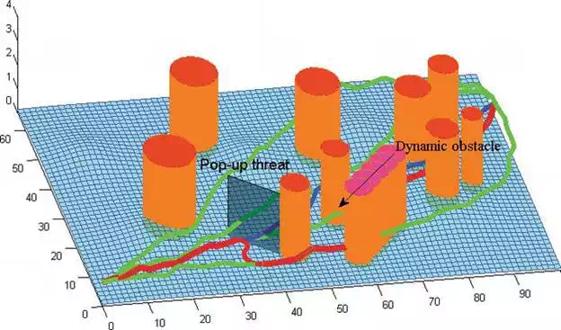
FIGURE 13.

The experiment of using MGAT for 3D emergency threat management case, where pop-up threat and moving threat are exist in the environment.

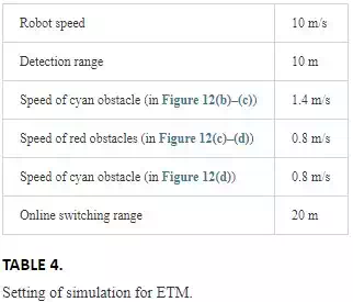
For all the experiments, we study the time efficiency of each switching to escape from current dangerous situation. For one moving threat avoiding (see in Figure 12(b)), the time needed to switch to other RAP is 0.0507 s, and the whole navigation duration is 13.14 s with 10 m/s speed. For two dynamic threats avoiding case (see in Figure 12(c)), the whole navigation time is 13.32 s, and the time spend to avoid the second threat is 0.0912 s. In scene 3, we designed a long duration for threat (see in Figure 12(d)). The two cyan threats disable the blue-path, thus robot has to switch for more times while tracking the dark path. The average time is no more than 0.15 s which can be decreased when implemented in robot’s platform with C++ implementation, and the whole navigation time is 13.5 s.

Conclusion

The main contribution of this paper is that an online EMT planner is proposed, where pop-up threat and moving obstacle happen during tracking the pre-planned path. We propose a new multiple path planning approach called MGART, which is improved based on GART, by introducing an ‘Extending Forbidden’ algorithm to shift the goal biased probability to neighbor branches around goal reached branch. The algorithm is shown to inherit the merits of GART and the ability of exploring in cluttered environments, and it guarantees asymptotically optimal and completeness. It is also shown that the algorithm can generate multiple paths without using variant cost principles, but only relying on the EFA threshold, thus it enables selection for online dynamical switching.

In the future, we would like to research on online visual positioning and environment perception topic, which is lack of discussion in this paper. We would like to enable cognitive sensing and autonomous for robots.