Artificial Intelligence in Geoscience and Remote Sensing

Artificial Intelligence in Geoscience and Remote Sensing

Introduction

Machine learning has recently found many applications in the geosciences and remote sensing. These applications range from bias correction to retrieval algorithms, from code acceleration to detection of disease in crops. As a broad subfield of artificial intelligence, machine learning is concerned with algorithms and techniques that allow computers to “learn”. The major focus of machine learning is to extract information from data automatically by computational and statistical methods.

Over the last decade there has been considerable progress in developing a machine learning methodology for a variety of Earth Science applications involving trace gases, retrievals, aerosol products, land surface products, vegetation indices, and most recently, ocean products (Yi and Prybutok, 1996, Atkinson and Tatnall, 1997, Carpenter et al., 1997, Comrie, 1997, Chevallier et al., 1998, Hyyppa et al., 1998, Gardner and Dorling, 1999, Lary et al., 2004, Lary et al., 2007, Brown et al., 2008, Lary and Aulov, 2008, Caselli et al., 2009, Lary et al., 2009). Some of this work has even received special recognition as a NASA Aura Science highlight (Lary et al., 2007) and commendation from the NASA MODIS instrument team (Lary et al., 2009). The two types of machine learning algorithms typically used are neural networks and support vector machines. In this chapter, we will review some examples of how machine learning is useful for Geoscience and remote sensing, these examples come from the author’s own research.

Typical Applications

One of the features that make machine-learning algorithms so useful is that they are “universal approximators”. They can learn the behaviour of a system if they are given a comprehensive set of examples in a training dataset. These examples should span as much of the parameter space as possible. Effective learning of the system’s behaviour can be achieved even if it is multivariate and non-linear. An additional useful feature is that we do not need to know a priori the functional form of the system as required by traditional least-squares fitting, in other words they are non-parametric, non-linear and multivariate learning algorithms.

The uses of machine learning to date have fallen into three basic categories which are widely applicable across all of the Geosciences and remote sensing, the first two categories use machine learning for its regression capabilities, the third category uses machine learning for its classification capabilities. We can characterize the three application themes are as follows: First, where we have a theoretical description of the system in the form of a deterministic model, but the model is computationally expensive. In this situation, a machine-learning “wrapper” can be applied to the deterministic model providing us with a “code accelerator”. A good example of this is in the case of atmospheric photochemistry where we need to solve a large coupled system of ordinary differential equations (ODEs) at a large grid of locations. It was found that applying a neural network wrapper to the system was able to provide a speed up of between a factor of 2 and 200 depending on the conditions. Second, when we do not have a deterministic model but we have data available enabling us to empirically learn the behaviour of the system. Examples of this would include: Learning inter-instrument bias between sensors with a temporal overlap, and inferring physical parameters from remotely sensed proxies. Third, machine learning can be used for classification, for example, in providing land surface type classifications. Support Vector Machines perform particularly well for classification problems. Now that we have an overview of the typical applications, the sections that follow will introduce two of the most powerful machine learning approaches, neural networks and support vector machines and then present a variety of examples.

Machine Learning

Neural Networks

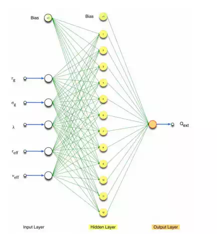
Neural networks are multivariate, non-parametric, ‘learning’ algorithms (Haykin, 1994, Bishop, 1995, 1998, Haykin, 2001a, Haykin, 2001b, 2007) inspired by biological neural networks. Computational neural networks (NN) consist of an interconnected group of artificial neurons that processes information in parallel using a connectionist approach to computation. A NN is a non-linear statistical data-modelling tool that can be used to model complex relationships between inputs and outputs or to find patterns in data. The basic computational element of a NN is a model neuron or node. A node receives input from other nodes, or an external source (e.g. the input variables). A schematic of an example NN is shown in Figure 1. Each input has an associated weight, w, that can be modified to mimic synaptic learning. The unit computes some function, f, of the weighted sum of its inputs:

Its output, in turn, can serve as input to other units. wij refers to the weight from unit j to unit i. The function f is the node’s activation or transfer function. The transfer function of a node defines the output of that node given an input or set of inputs. In the simplest case, f is the identity function, and the unit’s output is yi, this is called a linear node. However, non-linear sigmoid functions are often used, such as the hyperbolic tangent sigmoid transfer function and the log-sigmoid transfer function. Figure 1 shows an example feed-forward perceptron NN with five inputs, a single output, and twelve nodes in a hidden layer. A perceptron is a computer model devised to represent or simulate the ability of the brain to recognize and discriminate. In most cases, a NN is an adaptive system that changes its structure based on external or internal information that flows through the network during the learning phase.

When we perform neural network training, we want to ensure we can independently assess the quality of the machine learning ‘fit’. To insure this objective assessment we usually randomly split our training dataset into three portions, typically of 80%, 10% and 10%. The largest portion containing 80% of the dataset is used for training the neural network weights. This training is iterative, and on each training iteration we evaluate the current root mean square (RMS) error of the neural network output. The RMS error is calculated by using the second 10% portion of the data that was not used in the training. We use the RMS error and the way the RMS error changes with training iteration (epoch) to determine the convergence of our training. When the training is complete, we then use the final 10% portion of data as a totally independent validation dataset. This final 10% portion of the data is randomly chosen from the training dataset and is not used in either the training or RMS evaluation. We only use the neural network if the validation scatter diagram, which plots the actual data from validation portion against the neural network estimate, yields a straight-line graph with a slope very close to one and an intercept very close to zero. This is a stringent, independent and objective validation metric. The validation is global as the data is randomly selected over all data points available. For our studies, we typically used feed-forward back-propagation neural networks with a Levenberg-Marquardt back-propagation training algorithm (Levenberg, 1944, Marquardt, 1963, Moré, 1977, Marquardt, 1979).

Support Vector Machines

Support Vector Machines (SVM) are based on the concept of decision planes that define decision boundaries and were first introduced by Vapnik (Vapnik, 1995, 1998, 2000) and has subsequently been extended by others (Scholkopf et al., 2000, Smola and Scholkopf, 2004). A decision plane is one that separates between a set of objects having different class memberships. The simplest example is a linear classifier, i.e. a classifier that separates a set of objects into their respective groups with a line. However, most classification tasks are not that simple, and often more complex structures are needed in order to make an optimal separation, i.e., correctly classify new objects (test cases) on the basis of the examples that are available (training cases). Classification tasks based on drawing separating lines to distinguish between objects of different class memberships are known as hyperplane classifiers. SVMs are a set of related supervised learning methods used for classification and regression. Viewing input data as two sets of vectors in an n-dimensional space, an SVM will construct a separating hyperplane in that space, one that maximizes the margin between the two data sets. To calculate the margin, two parallel hyperplanes are constructed, one on each side of the separating hyperplane, which are “pushed up against” the two data sets. Intuitively, a good separation is achieved by the hyperplane that has the largest distance to the neighboring data points of both classes, since in general the larger the margin the better the generalization error of the classifier. We typically used the SVMs provided by LIBSVM (Fan et al., 2005, Chen et al., 2006).

Applications

Let us now consider some applications.

Bias Correction:

Atmospheric Chlorine Loading for Ozone Hole Research Critical in determining the speed at which the stratospheric ozone hole recovers is the total amount of atmospheric chlorine. Attributing changes in stratospheric ozone to changes in chlorine requires knowledge of the stratospheric chlorine abundance over time. Such attribution is central to international ozone assessments, such as those produced by the World Meteorological Organization (Wmo, 2006). However, we do not have continuous observations of all the key chlorine gases to provide such a continuous time series of stratospheric chlorine. To address this major limitation, we have devised a new technique that uses the long time series of available hydrochloric acid observations and neural networks to estimate the stratospheric chlorine (Cly) abundance (Lary et al., 2007). Knowledge of the distribution of inorganic chlorine Cly in the stratosphere is needed to attribute changes in stratospheric ozone to changes in halogens, and to assess the realism of chemistry-climate models (Eyring et al., 2006, Eyring et al., 2007, Waugh and Eyring, 2008). However, simultaneous measurements of the major inorganic chlorine species are rare (Zander et al., 1992, Gunson et al., 1994, Webster et al., 1994, Michelsen et al., 1996, Rinsland et al., 1996, Zander et al., 1996, Sen et al., 1999, Bonne et al., 2000, Voss et al., 2001, Dufour et al., 2006, Nassar et al., 2006). In the upper stratosphere, the situation is a little easier as Cly can be inferred from HCl alone (e.g., (Anderson et al., 2000, Froidevaux et al., 2006b, Santee et al., 2008)). Our new estimates of stratospheric chlorine using machine learning (Lary et al., 2007) work throughout the stratosphere and provide a much-needed critical test for current global models. This critical evaluation is necessary as there are significant differences in both the stratospheric chlorine and the timing of ozone recovery in the available model predictions. Hydrochloric acid is the major reactive chlorine gas throughout much of the atmosphere, and throughout much of the year. However, the observations of HCl that we do have (from UARS HALOE, ATMOS, SCISAT-1 ACE and Aura MLS) have significant biases relative to each other. We found that machine learning can also address the inter-instrument bias (Lary et al., 2007, Lary and Aulov, 2008). We compared measurements of HCl from the different instruments listed in Table 1. The Halogen Occultation Experiment (HALOE) provides the longest record of space based HCl observations. Figure 2 compares HALOE HCl with HCl observations from (a) the Atmospheric Trace Molecule Spectroscopy Experiment (ATMOS), (b) the Atmospheric Chemistry Experiment (ACE) and (c) the Microwave Limb Sounder (MLS).

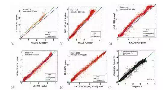
Fig. 2. Panels (a) to (d) show scatter plots of all contemporaneous observations of HCl made by HALOE, ATMOS, ACE and MLS Aura. In panels (a) to (c) HALOE is shown on the xaxis. Panel (e) correspond to panel (c) except that it uses the neural network ‘adjusted’ HALOE HCl values. Panel (f) shows the validation scatter diagram of the neural network estimate of Cly ≈ HCl + ClONO2 + ClO +HOCl versus the actual Cly for a totally independent data sample not used in training the neural network.

A consistent picture is seen in these plots: HALOE HCl measurements are lower than those from the other instruments. The slopes of the linear fits (relative scaling) are 1.05 for the HALOE-ATMOS comparison, 1.09 for the HALOE-MLS, and 1.18 for the HALOE-ACE. The offsets are apparent at the 525 K isentropic surface and above. Previous comparisons among HCl datasets reveal a similar bias for HALOE (Russell et al., 1996, Mchugh et al., 2005, Froidevaux et al., 2006a, Froidevaux et al., 2008). ACE and MLS HCl measurements are in much better agreement (Figure 2d). Note, the measurements agree within the stated observational uncertainties summarized in Table 1.

Table 1. The instruments and constituents used in constructing the Cly record from 1991- 2006. The uncertainties given are the median values calculated for each level 2 measurement profile and its uncertainty (both in mixing ratio) for all the observations made. The uncertainties are larger than usually quoted for MLS ClO because they reflect the single profile precision, which is improved by temporal and/or spatial averaging. The HALOE uncertainties are only estimates of random error and do not include any indications of overall accuracy.

To combine the above HCl measurements to form a continuous time series of HCl (and then Cly) from 1991 to 2006 it is necessary to account for the biases between data sets. A neural network is used to learn the mapping from one set of measurements onto another as a function of equivalent latitude and potential temperature. We consider two cases. In one case ACE HCl is taken as the reference and the HALOE and Aura HCl observations are adjusted to agree with ACE HCl. In the other case HALOE HCl is taken as the reference and the Aura and ACE HCl observations are adjusted to agree with HALOE HCl. In both cases we use equivalent latitude and potential temperature to produce average profiles. The purpose of the NN mapping is simply to learn the bias as a function of location, not to imply which instrument is correct. The precision of the correction using the neural network mapping is of the order of ±0.3 ppbv, as seen in Figure 2 (e) that shows the results when HALOE HCl measurements have been mapped into ACE measurements. The mapping has removed the bias between the measurements and has straightened out the ‘wiggles’ in 2 (c), i.e., the neural network has learned the equivalent PV latitude and potential temperature dependence of the bias between HALOE and MLS. The inter-instrument offsets are not constant in space or time, and are not a simple function of Cly.

So employing neural networks allows us to: Form a seamless record of HCl using observations from several space-borne instruments using neural networks. Provide an estimated of the associated inter-instrument bias. Infer Cly from HCl, and thereby provide a seamless record of Cly, the parameter needed for examining the ozone hole recovery. A similar use of machine learning has been made for Aerosol Optical Depths, the subject of the next sub-section.

Fig. 3. Cly average profiles between 30° and 60°N for October 2005, estimated by neural network calibrated to HALOE HCl (blue curve), estimated by neural network calibrated to ACE HCl (green), or from ACE observations of HCl, ClONO2, ClO, and HOCl (red crosses). In each case, the shaded range represents the total uncertainty; it includes the observational uncertainty, the representativeness uncertainty (the variability over the analysis grid cell), the neural network uncertainty. The vertical extent of this plot was limited to below 1000 K (≈35 km), as there is no ACE v2.2 ClO data for the upper altitudes. In addition, above ≈750 K (≈25 km), ClO constitutes a larger fraction of Cly (up to about 10%) and so the large uncertainties in ClO have greater effect.

Fig. 4. Panels (a) to (c) show October Cly time-series for the 525 K isentropic surface (≈20 km) and the 800 K isentropic surface (≈30 km). In each case the dark shaded range represents the total uncertainty in our estimate of Cly. This total uncertainty includes the observational uncertainty, the representativeness uncertainty (the variability over the analysis grid cell), the inter-instrument bias in HCl, the uncertainty associated with the neural network interinstrument correction, and the uncertainty associated with the neural network inference of Cly from HCl and CH4. The inner light shading depicts the uncertainty on Cly due to the interinstrument bias in HCl alone. The upper limit of the light shaded range corresponds to the estimate of Cly based on all the HCl observations calibrated by a neural network to agree with ACE v2.2 HCl. The lower limit of the light shaded range corresponds to the estimate of Cly based on all the HCl observations calibrated to agree with HALOE v19 HCl. Overlaid are lines showing the Cly based on age of air calculations (Newman et al., 2006). To minimize variations due to differing data coverage months with less than 100 observations of HCl in the equivalent latitude bin were left out of the time-series.

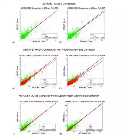
Fig. 5. Scatter diagram comparisons of Aerosol Optical Depth (AOD) from AERONET (xaxis) and MODIS (y-axis) as green circles overlaid with the ideal case of perfect agreement (blue line). The measurements shown in the comparison were made within half an hour of each other, with a great circle separation of less than 0.25° and with a solar zenith angle difference of less than 0.1°. The left hand column of plots is for MODIS Aqua and the right hand column of plots is for MODIS Terra. The first row shows the comparisons between AERONET and MODIS for the entire period of overlap between the MODIS and AERONET instruments from the launch of the MODIS instrument to the present. The second row shows the same comparison overlaid with the neural network correction as red circles. We note that the neural network bias correction makes a substantial improvement in the correlation coefficient with AERONET. An improvement from 0.86 to 0.96 for MODIS Aqua and an improvement from 0.84 to 0.92 for MODIS Terra. The third row shows the comparison overlaid with the support vector regression correction as red circles. We note that the support vector regression bias correction makes an even greater improvement in the correlation coefficient than the neural network correction. An improvement from 0.86 to 0.99 for MODIS Aqua and an improvement from 0.84 to 0.99 for MODIS Terra.

Bias Correction:

Aerosol Optical Depth As highlighted in the 2007 IPCC report on Climate Change, aerosol and cloud radiative effects remain the largest uncertainties in our understanding of climate change (Solomon et al., 2007). Over the past decade observations and retrievals of aerosol characteristics have been conducted from space-based sensors, from airborne instruments and from groundbased samplers and radiometers. Much effort has been directed at these data sets to collocate observations and retrievals, and to compare results. Ideally, when two instruments measure the same aerosol characteristic at the same time, the results should agree within well-understood measurement uncertainties. When inter-instrument biases exist, we would like to explain them theoretically from first principles. One example of this is the comparison between the aerosol optical depth (AOD) retrieved by the Moderate Resolution Imaging Spectroradiometer (MODIS) and the AOD measured by the Aerosol Robotics Network (AERONET). While progress has been made in understanding the biases between these two data sets, we still have an imperfect understanding of the root causes. (Lary et al., 2009) examined the efficacy of empirical machine learning algorithms for aerosol bias correction.

Machine learning approaches (Neural Networks and Support Vector Machines) were used by (Lary et al., 2009) to explore the reasons for a persistent bias between aerosol optical depth (AOD) retrieved from the MODerate resolution Imaging Spectroradiometer (MODIS) and the accurate ground-based Aerosol Robotics Network (AERONET). While this bias falls within the expected uncertainty of the MODIS algorithms, there is still room for algorithm improvement. The results of the machine learning approaches suggest a link between the MODIS AOD biases and surface type. From figure 5 we can see that machine learning algorithms were able to effectively adjust the AOD bias seen between the MODIS instruments and AERONET. Support vector machines performed the best improving the correlation coefficient between the AERONET AOD and the MODIS AOD from 0.86 to 0.99 for MODIS Aqua, and from 0.84 to 0.99 for MODIS Terra.

Key in allowing the machine learning algorithms to ‘correct’ the MODIS bias was provision of the surface type and other ancillary variables that explain the variance between MODIS and AERONET AOD. The provision of the ancillary variables that can explain the variance in the dataset is the key ingredient for the effective use of machine learning for bias correction. A similar use of machine learning has been made for vegetation indices, the subject of the next sub-section.

Bias Correction: Vegetation Indices

Consistent, long term vegetation data records are critical for analysis of the impact of global change on terrestrial ecosystems. Continuous observations of terrestrial ecosystems through time are necessary to document changes in magnitude or variability in an ecosystem (Tucker et al., 2001, Eklundh and Olsson, 2003, Slayback et al., 2003). Satellite remote sensing has been the primary way that scientists have measured global trends in vegetation, as the measurements are both global and temporally frequent. In order to extend measurements through time, multiple sensors with different design and resolution must be used together in the same time series. This presents significant problems as sensor band placement, spectral response, processing, and atmospheric correction of the observations can vary significantly and impact the comparability of the measurements (Brown et al., 2006). Even without differences in atmospheric correction, vegetation index values for the same target recorded under identical conditions will not be directly comparable because input reflectance values differ from sensor to sensor due to differences in sensor design (Teillet et al., 1997, Miura et al., 2006).

Several approaches have previously been taken to integrate data from multiple sensors. (Steven et al., 2003), for example, simulated the spectral response from multiple instruments and with simple linear equations created conversion coefficients to transform NDVI data from one sensor to another. Their analysis is based on the observation that the vegetation index is critically dependent on the spectral response functions of the instrument used to calculate it. The conversion formulas the paper presents cannot be applied to maximum value NDVI datasets because the weighting coefficients are land cover and dataset dependent, reducing their efficacy in mixed pixel situations (Steven et al., 2003). (Trishchenko et al., 2002) created a series of quadratic functions to correct for differences in the reflectance and NDVI to NOAA-9 AVHRR-equivalents (Trishchenko et al., 2002). Both the (Steven et al., 2003) and the (Trishchenko et al., 2002) approaches are land cover and dataset dependent and thus cannot be used on global datasets where multiple land covers are represented by one pixel. (Miura et al., 2006) used hyper-spectral data to investigate the effect of different spectral response characteristics between MODIS and AVHRR instruments on both the reflectance and NDVI data, showing that the precise characteristics of the spectral response had a large effect on the resulting vegetation index. The complex patterns and dependencies on spectral band functions were both land cover dependent and strongly non-linear, thus we see that an exploration of a nonlinear approach may be fruitful.

(Brown et al., 2008) experimented with powerful, non-linear neural networks to identify and remove differences in sensor design and variable atmospheric contamination from the AVHRR NDVI record in order to match the range and variance of MODIS NDVI without removing the desired signal representing the underlying vegetation dynamics. Neural networks are ‘data transformers’ (Atkinson and Tatnall, 1997), where the objective is to associate the elements of one set of data to the elements in another. Relationships between the two datasets can be complex and the two datasets may have different statistical distributions. In addition, neural networks incorporate a priori knowledge and realistic physical constraints into the analysis, enabling a transformation from one dataset into another through a set of weighting functions (Atkinson and Tatnall, 1997). This transformation incorporates additional input data that may account for differences between the two datasets.

The objective of (Brown et al., 2008) was to demonstrate the viability of neural networks as a tool to produce a long term dataset based on AVHRR NDVI that has the data range and statistical distribution of MODIS NDVI. Previous work has shown that the relationship between AVHRR and MODIS NDVI is complex and nonlinear (Gallo et al., 2003, Brown et al., 2006, Miura et al., 2006), thus this problem is well suited to neural networks if appropriate inputs can be found. The influence of the variation of atmospheric contamination of the AVHRR data through time was explored by using observed atmospheric water vapor from the Total Ozone Mapping Spectrometer (TOMS) instrument during the overlap period 2000-2004 and back to 1985. Examination of the resulting MODIS fitted AVHRR dataset both during the overlap period and in the historical dataset will enable an evaluation of the efficacy of the neural net approach compared to other approaches to merge multiple-sensor NDVI datasets.

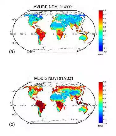
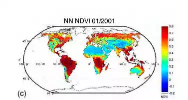
Fig. 6. A comparison of the NDVI from AVHR (panel a), MODIS (panel p), and then a reconstruction of MODIS using AVHRR and machine learning (panel c). We note that the machine learning can successfully account for the large differences that are found between AVHRR and MODIS.

Remote sensing datasets are the result of a complex interaction between the design of a sensor, the spectral response function, stability in orbit, the processing of the raw data, compositing schemes, and post-processing corrections for various atmospheric effects including clouds and aerosols. The interaction between these various elements is often non-linear and non-additive, where some elements increase the vegetation signal to noise ratio (compositing, for example) and others reduce it (clouds and volcanic aerosols) (Los, 1998). Thus, although other authors have used simulated data to explore the relationship between AVHRR and MODIS (Trishchenko et al., 2002, Van Leeuwen et al., 2006), these techniques are not directly useful in producing a sensorindependent vegetation dataset that can be used by data users in the near term.

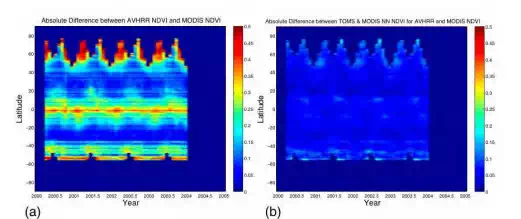
Fig. 7. Panel (a) shows a time-series from 2000 to 2003 of the zonal mean (averaged per latitude) difference between the AVHRR and MODIS NDVIs, this highlights that significant differences exist between the two data products. Panel (b) shows a time series over the same period after the machine learning has been used to “cross-calibrate” AVHRR as MODIS, showing that the machine learning has effectively learnt how to cross-calibrate the instruments.

There are substantial differences between the processed vegetation data from AVHRR and MODIS. (Brown et al., 2008) showed that neural networks are an effective way to have a long data record that utilizes all available data back to 1981 by providing a practical way of incorporating the AVHRR data into a continuum of observations that include both MODIS and VIIRS. The results (Brown et al., 2008) showed that the TOMS data record on clouds, ozone and aerosols can be used to identify and remove sensor-specific atmospheric contaminants that differentially affect the AVHRR over MODIS. Other sensor-related effects, particularly those of changing BRDF, viewing angle, illumination, and other effects that are not accounted for here, remain important sources of additional variability. Although this analysis has not produced a dataset with identical properties to MODIS, it has demonstrated that a neural net approach can remove most of the atmospheric-related aspects of the differences between the sensors, and match the mean, standard deviation and range of the two sensors. A similar technique can be used for the VIIRS sensor once the data is released.

Figure 6 shows a comparison of the NDVI from AVHR (panel a), MODIS (panel p), and then a reconstruction of MODIS using AVHRR and machine learning (panel c). Figure 7 (a) shows a time-series from 2000 to 2003 of the zonal mean difference between the AVHRR and MODIS NDVIs, this highlights that significant differences exist between the two data products. Panel (b) shows a time series over the same period after the machine learning has been used to “cross-calibrate” AVHRR as MODIS, illustrating that the machine learning has effectively learnt how to cross-calibrate the instruments.

So far, we have seen three examples of using machine learning for bias correction (constituent biases, aerosol optical depth biases and vegetation index biases), and one example of using machine learning to infer a useful proxy from remotely sensed data (Cly from HCl). Let us look at one more example of inferring proxies from existing remotely sensed data before moving onto consider using machine learning for code acceleration.

Inferring Proxies: Tracer Correlations

The spatial distributions of atmospheric trace constituents are in general dependent on both chemistry and transport. Compact correlations between long-lived species are well-observed features in the middle atmosphere. The correlations exist for all long-lived tracers - not just those that are chemically related - due to their transport by the general circulation of the atmosphere. The tight relationships between different constituents have led to many analyses using measurements of one tracer to infer the abundance of another tracer. Using these correlations is also as a diagnostic of mixing and can distinguish between air-parcels of different origins. Of special interest are the so-called ‘long-lived’ tracers: constituents such as nitrous oxide (N2O), methane (CH4), and the chlorofluorocarbons (CFCs) that have long lifetimes (many years) in the troposphere and lower stratosphere, but are destroyed rapidly in the middle and upper stratosphere.

The correlations are spatially and temporally dependent. For example, there is a ‘compactrelation’ regime in the lower part of the stratosphere and an ‘altitude-dependent' regime above this. In the compact-relation region, the abundance of one tracer is uniquely determined by the value of the other tracer, without regard to other variables such as latitude or altitude. In the altitude-dependent regime, the correlation generally shows significant variation with altitude. A family of correlations usually achieves the description of such spatially and temporally dependent correlations. However, a single neural network is a natural and effective alternative. The motivation for this case study was preparation for a long-term chemical assimilation of Upper Atmosphere Research Satellite (UARS) data starting in 1991 and coming up to the present. For this period, we have continuous version 19 data from the Halogen Occultation Experiment (HALOE) but not observations of N2O as both ISAMS and CLAES failed. In addition, we would like to constrain the total amount of reactive nitrogen, chlorine, and bromine in a self-consistent way (i.e. the correlations between the long-lived tracers is preserved). Tracer correlations provide a means to do this by using HALOE CH4 observations. Machine learning is ideally suited to describe the spatial and temporal dependence of tracertracer correlations. The neural network performs well even in regions where the correlations are less compact and normally a family of correlation curves would be required. For example, the methane CH4-N2O correlation can be well described using a neural network (Lary et al., 2004) trained with the latitude, pressure, time of year, and CH4 volume mixing ratio (v.m.r.). Lary et al. (2004) used a neural network to reproduce the CH4-N2O correlation with a correlation coefficient between simulated and training values of 0.9995. Such an accurate representation of tracer-tracer correlations allows more use to be made of long-term datasets to constrain chemical models. For example, the Halogen Occultation Experiment (HALOE) that continuously observed CH4 (but not N2O) from 1991 until 2005.

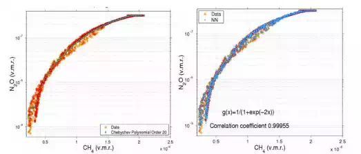
Fig. 8. Panel (a) shows the global N2O-CH4 correlation for an entire year, after evaluating the efficacy of 3,000 different functional forms for parametric fits, we overlaid the best, an order 20 Chebyshev Polynomial. However, this still does not account for the multi-variate nature of the problem exhibited by the ‘cloud’ of points rather than a compact ‘curve’ or ‘line’. However, in panel (b) we can see that a neural network is able to account for the non-linear and multi-variate aspects, the training dataset exhibited a ‘cloud’ of points, the neural network fit reproduces a ‘cloud’ of points. The most important factor in producing a ‘spread’ in the correlations is the strong altitude dependence of the N2O-CH4 correlation.

Figure 8 (a) shows the global N2O-CH4 correlation for an entire year, after evaluating the efficacy of 3,000 different functional forms for parametric fits, we overlaid the best, an order 20 Chebyshev Polynomial. However, this still does not account for the multi-variate nature of the problem exhibited by the ‘cloud’ of points rather than a compact ‘curve’ or ‘line’. However, in Figure 8 (b) we can see that a neural network is able to account for the non-linear and multivariate aspects, the training dataset exhibited a ‘cloud’ of points, the neural network fit reproduces a ‘cloud’ of points. The most important factor in producing a ‘spread’ in the correlations is the strong altitude dependence of the N2O-CH4 correlation.

Code Acceleration: Example from Ordinary Differential Equation Solvers

There are many applications in the Geosciences and remote sensing which are computationally expensive. Machine learning can be very effective in accelerating components of these calculations. We can readily create training datasets for these applications using the very models we would like to accelerate.

The first example for which we found this effective was solving ordinary differential equations. An adequate photochemical mechanism to describe the evolution of ozone in the upper troposphere and lower stratosphere (UT/LS) in a computational model involves a comprehensive treatment of reactive nitrogen, hydrogen, halogens, hydrocarbons, and interactions with aerosols. Describing this complex interaction is computationally expensive, and applications are limited by the computational burden. Simulations are often made tractable by using a coarser horizontal resolution than would be desired or by reducing the interactions accounted for in the photochemical mechanism. These compromises also limit the scientific applications. Machine learning algorithms offer a means to obtain a fast and accurate solution to the stiff ordinary differential equations that comprise the photochemical calculations, thus making high-resolution simulations including the complete photochemical mechanism much more tractable.

For the sake of an example, a 3D model of atmospheric chemistry and transport, the GMICOMBO model, can use 55 vertical levels and a 4° latitude x 5° longitude grid and 125 species. With 15-minute time steps the chemical ODE solver is called 119,750,400 times in simulating just one week. If the simulation is for a year then the ODE solver needs to be called 6,227,020,800 (or 6x109) times. If the spatial and temporal resolution is doubled then the chemical ODE solver needs to be called a staggering 2.5x1010 times to simulate a year. This represents a major computational cost in simulating a constituent’s spatial and temporal evolution. The ODEs solved at adjacent grid cells and time steps are very similar. Therefore, if the simulations from one grid cell and time step could be used to speed up the simulation for adjacent grid cells and subsequent time steps, we would have a strategy to dramatically decrease the computational cost of our simulations.

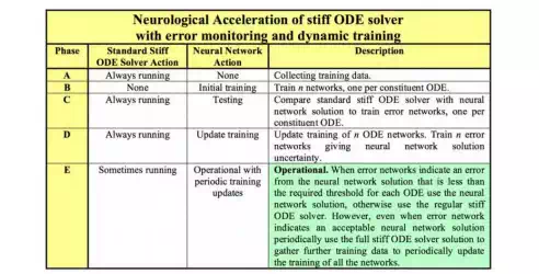
Figure 9 shows the strategy that we used for applying a neural wrapper to accelerate the ODE solver. Figure 10 shows some example results for ozone after using a neural wrapper around an atmospheric chemistry ODE solver. The x-axis shows the actual ozone abundance as a volume mixing ratio (vmr) using the regular ODE solver without neural networks. The y-axis shows the ozone vmr inferred using the neural network solution. It can be seen that we have excellent agreement between the two solutions with a correlation coefficient of 1. The neural network has learned the behaviour of the ozone ODE very well. Without the adaptive error control the acceleration could be up to 200 times, with the full adaptive error control the acceleration was less, but usually at least a factor of two. Similarly, in Figure 11 the two panels below show the results for formaldehyde (HCHO) in the GMI model. The left panel shows the solution with SMVGear for level 1 at 01:00 UT and the right panel shows the corresponding solution using the neural network. As one would hope, the two results are almost indistinguishable.

Fig. 10. Example results for using a neural wrapper around an atmospheric chemistry ODE solver. The x-axis shows the actual ozone v.m.r. using the regular ODE solver without neural networks. The y-axis shows the ozone v.m.r. inferred using the neural network solution. It can be seen that we have excellent agreement between the two solutions with a correlation coefficient of 1. The neural network has learned the behaviour of the ozone ODE very well.

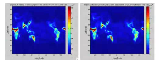
Fig. 11. The two panels below show the results for formaldehyde (HCHO) in the GMI model. The left panel shows the solution with SMVGear for level 1 at 01:00 UT and the right panel shows the corresponding solution using the neural network. As one would hope, the two results are almost indistinguishable.

Classification: Example from Detecting Drought Stress and Infection in Cacao

The source of chocolate, theobroma cacao (cacao), is an understory tropical tree (Wood, 2001). Cacao is intolerant to drought (Belsky and Siebert, 2003), and yields and production patterns are severely affected by periodic droughts and seasonal rainfall patterns. (Bae et al., 2008) studied the molecular response of cacao to drought and have identified several genes responsive to drought stress (Bailey et al., 2006). They have also been studying the response of cacao to colonization by an endophytic isolates of Trichoderma including Trichoderma hamatum, DIS 219b (Bailey et al., 2006). One of the benefits to colonization Trichoderma hamatum isolate DIS 219b is tolerance to drought as mediated through plant growth promotion, specifically enhanced root growth (Bae et al., 2008).

In characterizing the drought response of cacao considerable variation was observed in the response of individual seedlings depending upon the degree of drought stress applied (Bae et al., 2008). In addition, although colonization by DIS 219b delayed the drought response, direct effects of DIS 219b on cacao gene expression in the absence of drought were difficult to identify (Bae et al., 2008). The complexity of the DIS 219b/cacao plant microbe interaction overlaid on cacao’s response to drought makes the system of looking at individual genes as a marker for either drought or endophyte inefficient.

There would be considerable utility in reliably predicting drought and endophyte stress from complex gene expression patterns, particularly as the endophyte lives within the plant without causing apparent phenotypic changes in the plant. Machine‐learning models offer the possibility of highly accurate, automated predictions of plant stress from a variety of causes that may otherwise go undetected or be obscured by the complexity of plant responses to multiple environmental factors, to be considered status quo for plants in nature. We examined the ability of five different machine‐learning approaches to predict drought stress and endophyte colonization in cacao: a naive Bayes classifier, decision trees (DTs), neural networks (NN), neuro-fuzzy inference (NFI), and support vector machine (SVM) classification. The results provided some support for the accuracy of machine-learning models in discerning endophyte colonization and drought stress. The best performance was by the neuro-fuzzy inference system and the support vector classifier that correctly identified 100% of the drought and endophyte stress samples. Of the two, the approaches the support vector classifier is likely to have the best generalization (wider applicability to data not previously seen in the training process). Why did the SVM model outperform the four other machine learning approaches? We noted earlier that SVMs construct separating hyperplanes that maximize the margins between the different clusters in the training data set (the vectors that constrain the width of the margin are the support vectors). A good separation is achieved by those hyperplanes providing the largest distance between neighbouring classes, and in general, the larger the margin the better the generalization of the classifier.

When the points in neighbouring classes are separated by a nonlinear dividing line, rather than fitting nonlinear curves to the data, SVMs use a kernel function to map the data into a different space where a hyperplane can once more be used to do the separation. The kernel function may transform the data into a higher dimensional space to make it possible to perform the separation. The concept of a kernel mapping function is very powerful. It allows SVM models to perform separations even with very complex boundaries. Hence, we infer that, in the present application, the SVM model algorithmic process utilizes higher dimensional space to achieve superior predictive power.

For classification, the SVM algorithmic process offers an important advantage compared with neural network approaches. Specifically, neural networks can suffer from multiple local minima; in contrast, the solution to a support vector machine is global and unique. This characteristic may be partially attributed to the development process of these algorithms; SVMs were developed in the reverse order to the development of neural networks. SVMs evolved from the theory to implementation and experiments; neural networks followed a more heuristic path, from applications and extensive experimentation to theory.

In handling this data using traditional methods where individual gene responses are characterized as treatment effects, it was especially difficult to sort out direct effects of endophyte on gene expression over time or at specific time points. The differences between the responses of non-stressed plants with or without the endophyte were small and, after the zero time point, were highly variable. The general conclusion from this study was that colonization of cacao seedlings by the endophyte enhanced root growth resulting in increased drought tolerance but the direct effects of endophyte on cacao gene expression at the time points studied were minimal. Yet the neuro-fuzzy inference and support vector classification methods of analysis were able identify samples receiving these treatments correctly.

In this system, each gene in the plants genome is a potential sensor for the applied stress or treatment. It is not necessary that the genes response be significant in itself in determining the outcome of the plants response or that it be consistent in time or level of response. Since multiple genes are used in characterizing the response it is always the relative response in terms of the many other changes that are occurring at the same time as influenced by uncontrolled changes in the system that is important. With this study the treatments were controlled but variation in the genetic make up of each seedling (they were from segregating open pollinated seed) and minute differences in air currents within the chamber, soil composition, colonization levels, microbial populations within each pot and seedling, and even exact watering levels at each time point, all likely contributed to creating uncontrolled variation in the plants response to what is already a complex reaction to multiple factors (drought and endophyte). This type of variation makes accessing treatment responses using single gene approaches difficult and the prediction of cause due to effect in open systems almost impossible in complex systems.

Future Directions

We have seen the utility of machine learning for a suite of very diverse applications. These applications often help us make better use of existing data in a variety of ways. In parallel to the success of machine learning we also have the rapid development of publically available web services. So it is timely to combine both approached by providing online services that use machine learning for intelligent data fusion as part of a workflow that allows us to cross-calibrate multiple datasets. This obviously requires care to ensure the appropriate of datasets. However, if done carefully, this could greatly facilitate the production of seamless multi-year global records for a host of Earth science applications.

When it comes to dealing with inter-instrument biases in a consistent manner there is currently a gap in many space agencies’ Earth science information systems. This could be addressed by providing an extensible and reusable open source infrastructure that gap that could be reused for multiple projects. A clear need for such an infrastructure would be for NASA’s future Decadal Survey missions.

Summary

Machine learning has recently found many applications in the geosciences and remote sensing. These applications range from bias correction to retrieval algorithms, from code acceleration to detection of disease in crops. Machine-learning algorithms can act as “universal approximators”, they can learn the behaviour of a system if they are given a comprehensive set of examples in a training dataset. Effective learning of the system’s behaviour can be achieved even if it is multivariate and non-linear. An additional useful feature is that we do not need to know a priori the functional form of the system as required by traditional least-squares fitting, in other words they are non-parametric, non-linear and multivariate learning algorithms.