
The hinge loss function has many extensions, often the subject of investigation with SVM models.
A popular extension is called the squared hinge loss that simply calculates the square of the score hinge loss. It has the effect of smoothing the surface of the error function and making it numerically easier to work with.
If using a hinge loss does result in better performance on a given binary classification problem, is likely that a squared hinge loss may be appropriate.
As with using the hinge loss function, the target variable must be modified to have values in the set {-1, 1}.
1 2 | # change y from {0,1} to {-1,1} y[where(y == 0)] = -1 |
The squared hinge loss can be specified as ‘squared_hinge‘ in the compile()function when defining the model.

1 | model.compile(loss='squared_hinge', optimizer=opt, metrics=['accuracy']) |
And finally, the output layer must use a single node with a hyperbolic tangent activation function capable of outputting continuous values in the range [-1, 1].

1 | model.add(Dense(1, activation='tanh')) |
The complete example of an MLP with the squared hinge loss function on the two circles binary classification problem is listed below.

1 2 3 4 5 6 7 8 9 10 11 12 13 14 15 16 17 18 19 20 21 22 23 24 25 26 27 28 29 30 31 32 33 34 35 36 37 38 39 40 | # mlp for the circles problem with squared hinge loss from sklearn.datasets import make_circles from keras.models import Sequential from keras.layers import Dense from keras.optimizers import SGD from matplotlib import pyplot from numpy import where # generate 2d classification dataset X, y = make_circles(n_samples=1000, noise=0.1, random_state=1) # change y from {0,1} to {-1,1} y[where(y == 0)] = -1 # split into train and test n_train = 500 trainX, testX = X[:n_train, :], X[n_train:, :] trainy, testy = y[:n_train], y[n_train:] # define model model = Sequential() model.add(Dense(50, input_dim=2, activation='relu', kernel_initializer='he_uniform')) model.add(Dense(1, activation='tanh')) opt = SGD(lr=0.01, momentum=0.9) model.compile(loss='squared_hinge', optimizer=opt, metrics=['accuracy']) # fit model history = model.fit(trainX, trainy, validation_data=(testX, testy), epochs=200, verbose=0) # evaluate the model _, train_acc = model.evaluate(trainX, trainy, verbose=0) _, test_acc = model.evaluate(testX, testy, verbose=0) print('Train: %.3f, Test: %.3f' % (train_acc, test_acc)) # plot loss during training pyplot.subplot(211) pyplot.title('Loss') pyplot.plot(history.history['loss'], label='train') pyplot.plot(history.history['val_loss'], label='test') pyplot.legend() # plot accuracy during training pyplot.subplot(212) pyplot.title('Accuracy') pyplot.plot(history.history['acc'], label='train') pyplot.plot(history.history['val_acc'], label='test') pyplot.legend() pyplot.show() |
Running the example first prints the classification accuracy for the model on the train and test datasets.
Given the stochastic nature of the training algorithm, your specific results may vary. Try running the example a few times.
In this case, we can see that for this problem and the chosen model configuration, the hinge squared loss may not be appropriate, resulting in classification accuracy of less than 70% on the train and test sets.

1 | Train: 0.682, Test: 0.646 |
A figure is also created showing two line plots, the top with the squared hinge loss over epochs for the train (blue) and test (orange) dataset, and the bottom plot showing classification accuracy over epochs.
The plot of loss shows that indeed, the model converged, but the shape of the error surface is not as smooth as other loss functions where small changes to the weights are causing large changes in loss.
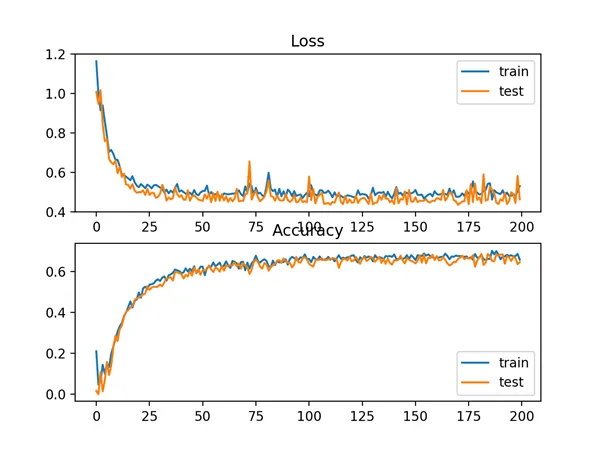
Line Plots of Squared Hinge Loss and Classification Accuracy over Training Epochs on the Two Circles Binary Classification Problem