
An alternative to cross-entropy for binary classification problems is the hinge loss function, primarily developed for use with Support Vector Machine (SVM) models.
It is intended for use with binary classification where the target values are in the set {-1, 1}.
The hinge loss function encourages examples to have the correct sign, assigning more error when there is a difference in the sign between the actual and predicted class values.
Reports of performance with the hinge loss are mixed, sometimes resulting in better performance than cross-entropy on binary classification problems.
Firstly, the target variable must be modified to have values in the set {-1, 1}.
1 2 | # change y from {0,1} to {-1,1} y[where(y == 0)] = -1 |
The hinge loss function can then be specified as the ‘hinge‘ in the compile function.

1 | model.compile(loss='hinge', optimizer=opt, metrics=['accuracy']) |
Finally, the output layer of the network must be configured to have a single node with a hyperbolic tangent activation function capable of outputting a single value in the range [-1, 1].

1 | model.add(Dense(1, activation='tanh')) |
The complete example of an MLP with a hinge loss function for the two circles binary classification problem is listed below.

1 2 3 4 5 6 7 8 9 10 11 12 13 14 15 16 17 18 19 20 21 22 23 24 25 26 27 28 29 30 31 32 33 34 35 36 37 38 39 40 | # mlp for the circles problem with hinge loss from sklearn.datasets import make_circles from keras.models import Sequential from keras.layers import Dense from keras.optimizers import SGD from matplotlib import pyplot from numpy import where # generate 2d classification dataset X, y = make_circles(n_samples=1000, noise=0.1, random_state=1) # change y from {0,1} to {-1,1} y[where(y == 0)] = -1 # split into train and test n_train = 500 trainX, testX = X[:n_train, :], X[n_train:, :] trainy, testy = y[:n_train], y[n_train:] # define model model = Sequential() model.add(Dense(50, input_dim=2, activation='relu', kernel_initializer='he_uniform')) model.add(Dense(1, activation='tanh')) opt = SGD(lr=0.01, momentum=0.9) model.compile(loss='hinge', optimizer=opt, metrics=['accuracy']) # fit model history = model.fit(trainX, trainy, validation_data=(testX, testy), epochs=200, verbose=0) # evaluate the model _, train_acc = model.evaluate(trainX, trainy, verbose=0) _, test_acc = model.evaluate(testX, testy, verbose=0) print('Train: %.3f, Test: %.3f' % (train_acc, test_acc)) # plot loss during training pyplot.subplot(211) pyplot.title('Loss') pyplot.plot(history.history['loss'], label='train') pyplot.plot(history.history['val_loss'], label='test') pyplot.legend() # plot accuracy during training pyplot.subplot(212) pyplot.title('Accuracy') pyplot.plot(history.history['acc'], label='train') pyplot.plot(history.history['val_acc'], label='test') pyplot.legend() pyplot.show() |
Running the example first prints the classification accuracy for the model on the train and test dataset.
Given the stochastic nature of the training algorithm, your specific results may vary. Try running the example a few times.
In this case, we can see slightly worse performance than using cross-entropy, with the chosen model configuration with less than 80% accuracy on the train and test sets.

1 | Train: 0.792, Test: 0.740 |
A figure is also created showing two line plots, the top with the hinge loss over epochs for the train (blue) and test (orange) dataset, and the bottom plot showing classification accuracy over epochs.
The plot of hinge loss shows that the model has converged and has reasonable loss on both datasets. The plot of classification accuracy also shows signs of convergence, albeit at a lower level of skill than may be desirable on this problem.
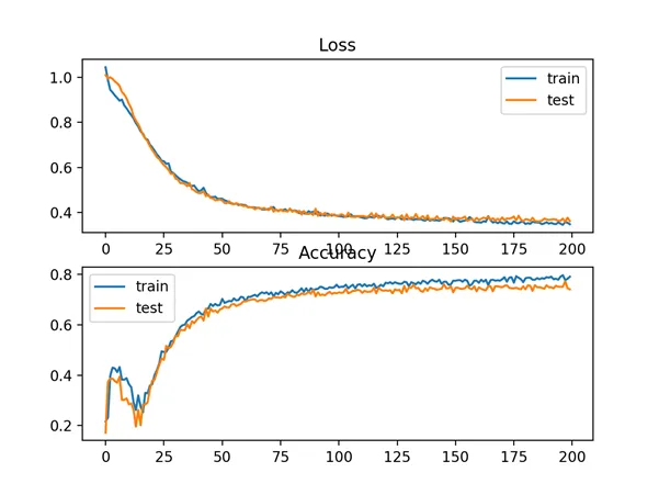
Line Plots of Hinge Loss and Classification Accuracy over Training Epochs on the Two Circles Binary Classification Problem