
Cross-entropy is the default loss function to use for binary classification problems.
It is intended for use with binary classification where the target values are in the set {0, 1}.
Mathematically, it is the preferred loss function under the inference framework of maximum likelihood. It is the loss function to be evaluated first and only changed if you have a good reason.
Cross-entropy will calculate a score that summarizes the average difference between the actual and predicted probability distributions for predicting class 1. The score is minimized and a perfect cross-entropy value is 0.
Cross-entropy can be specified as the loss function in Keras by specifying ‘binary_crossentropy‘ when compiling the model.
1 | model.compile(loss='binary_crossentropy', optimizer=opt, metrics=['accuracy']) |
The function requires that the output layer is configured with a single node and a ‘sigmoid‘ activation in order to predict the probability for class 1.
1 | model.add(Dense(1, activation='sigmoid')) |
The complete example of an MLP with cross-entropy loss for the two circles binary classification problem is listed below.

1 2 3 4 5 6 7 8 9 10 11 12 13 14 15 16 17 18 19 20 21 22 23 24 25 26 27 28 29 30 31 32 33 34 35 36 37 | # mlp for the circles problem with cross entropy loss from sklearn.datasets import make_circles from keras.models import Sequential from keras.layers import Dense from keras.optimizers import SGD from matplotlib import pyplot # generate 2d classification dataset X, y = make_circles(n_samples=1000, noise=0.1, random_state=1) # split into train and test n_train = 500 trainX, testX = X[:n_train, :], X[n_train:, :] trainy, testy = y[:n_train], y[n_train:] # define model model = Sequential() model.add(Dense(50, input_dim=2, activation='relu', kernel_initializer='he_uniform')) model.add(Dense(1, activation='sigmoid')) opt = SGD(lr=0.01, momentum=0.9) model.compile(loss='binary_crossentropy', optimizer=opt, metrics=['accuracy']) # fit model history = model.fit(trainX, trainy, validation_data=(testX, testy), epochs=200, verbose=0) # evaluate the model _, train_acc = model.evaluate(trainX, trainy, verbose=0) _, test_acc = model.evaluate(testX, testy, verbose=0) print('Train: %.3f, Test: %.3f' % (train_acc, test_acc)) # plot loss during training pyplot.subplot(211) pyplot.title('Loss') pyplot.plot(history.history['loss'], label='train') pyplot.plot(history.history['val_loss'], label='test') pyplot.legend() # plot accuracy during training pyplot.subplot(212) pyplot.title('Accuracy') pyplot.plot(history.history['acc'], label='train') pyplot.plot(history.history['val_acc'], label='test') pyplot.legend() pyplot.show() |
Running the example first prints the classification accuracy for the model on the train and test dataset.
Given the stochastic nature of the training algorithm, your specific results may vary. Try running the example a few times.
In this case, we can see that the model learned the problem reasonably well, achieving about 83% accuracy on the training dataset and about 85% on the test dataset. The scores are reasonably close, suggesting the model is probably not over or underfit.

1 | Train: 0.836, Test: 0.852 |
A figure is also created showing two line plots, the top with the cross-entropy loss over epochs for the train (blue) and test (orange) dataset, and the bottom plot showing classification accuracy over epochs.
The plot shows that the training process converged well. The plot for loss is smooth, given the continuous nature of the error between the probability distributions, whereas the line plot for accuracy shows bumps, given examples in the train and test set can ultimately only be predicted as correct or incorrect, providing less granular feedback on performance.
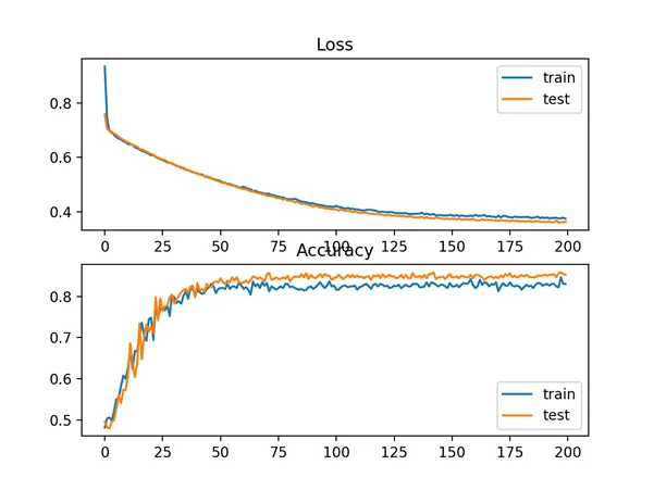
Line Plots of Cross Entropy Loss and Classification Accuracy over Training Epochs on the Two Circles Binary Classification Problem