
Binary classification are those predictive modeling problems where examples are assigned one of two labels.
The problem is often framed as predicting a value of 0 or 1 for the first or second class and is often implemented as predicting the probability of the example belonging to class value 1.
In this section, we will investigate loss functions that are appropriate for binary classification predictive modeling problems.
We will generate examples from the circles test problem in scikit-learn as the basis for this investigation. The circles problem involves samples drawn from two concentric circles on a two-dimensional plane, where points on the outer circle belong to class 0 and points for the inner circle belong to class 1. Statistical noise is added to the samples to add ambiguity and make the problem more challenging to learn.
We will generate 1,000 examples and add 10% statistical noise. The pseudorandom number generator will be seeded with the same value to ensure that we always get the same 1,000 examples.
1 2 | # generate circles X, y = make_circles(n_samples=1000, noise=0.1, random_state=1) |
We can create a scatter plot of the dataset to get an idea of the problem we are modeling. The complete example is listed below.

1 2 3 4 5 6 7 8 9 10 11 12 | # scatter plot of the circles dataset with points colored by class from sklearn.datasets import make_circles from numpy import where from matplotlib import pyplot # generate circles X, y = make_circles(n_samples=1000, noise=0.1, random_state=1) # select indices of points with each class label for i in range(2): samples_ix = where(y == i) pyplot.scatter(X[samples_ix, 0], X[samples_ix, 1], label=str(i)) pyplot.legend() pyplot.show() |
Running the example creates a scatter plot of the examples, where the input variables define the location of the point and the class value defines the color, with class 0 blue and class 1 orange.
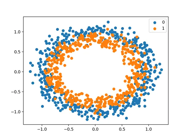
Scatter Plot of Dataset for the Circles Binary Classification Problem
The points are already reasonably scaled around 0, almost in [-1,1]. We won’t rescale them in this case.
The dataset is split evenly for train and test sets.

1 2 3 4 | # split into train and test n_train = 500 trainX, testX = X[:n_train, :], X[n_train:, :] trainy, testy = y[:n_train], y[n_train:] |
A simple MLP model can be defined to address this problem that expects two inputs for the two features in the dataset, a hidden layer with 50 nodes, a rectified linear activation function and an output layer that will need to be configured for the choice of loss function.

1 2 3 4 | # define model model = Sequential() model.add(Dense(50, input_dim=2, activation='relu', kernel_initializer='he_uniform')) model.add(Dense(1, activation='...')) |
The model will be fit using stochastic gradient descent with the sensible default learning rate of 0.01 and momentum of 0.9.

1 2 | opt = SGD(lr=0.01, momentum=0.9) model.compile(loss='...', optimizer=opt, metrics=['accuracy']) |
We will fit the model for 200 training epochs and evaluate the performance of the model against the loss and accuracy at the end of each epoch so that we can plot learning curves.

1 2 | # fit model history = model.fit(trainX, trainy, validation_data=(testX, testy), epochs=200, verbose=0) |
Now that we have the basis of a problem and model, we can take a look evaluating three common loss functions that are appropriate for a binary classification predictive modeling problem.
Although an MLP is used in these examples, the same loss functions can be used when training CNN and RNN models for binary classification.