
On some regression problems, the distribution of the target variable may be mostly Gaussian, but may have outliers, e.g. large or small values far from the mean value.
The Mean Absolute Error, or MAE, loss is an appropriate loss function in this case as it is more robust to outliers. It is calculated as the average of the absolute difference between the actual and predicted values.
The model can be updated to use the ‘mean_absolute_error‘ loss function and keep the same configuration for the output layer.
1 | model.compile(loss='mean_absolute_error', optimizer=opt, metrics=['mse']) |
The complete example using the mean absolute error as the loss function on the regression test problem is listed below.

1 2 3 4 5 6 7 8 9 10 11 12 13 14 15 16 17 18 19 20 21 22 23 24 25 26 27 28 29 30 31 32 33 34 35 36 37 38 39 40 41 | # mlp for regression with mae loss function from sklearn.datasets import make_regression from sklearn.preprocessing import StandardScaler from keras.models import Sequential from keras.layers import Dense from keras.optimizers import SGD from matplotlib import pyplot # generate regression dataset X, y = make_regression(n_samples=1000, n_features=20, noise=0.1, random_state=1) # standardize dataset X = StandardScaler().fit_transform(X) y = StandardScaler().fit_transform(y.reshape(len(y),1))[:,0] # split into train and test n_train = 500 trainX, testX = X[:n_train, :], X[n_train:, :] trainy, testy = y[:n_train], y[n_train:] # define model model = Sequential() model.add(Dense(25, input_dim=20, activation='relu', kernel_initializer='he_uniform')) model.add(Dense(1, activation='linear')) opt = SGD(lr=0.01, momentum=0.9) model.compile(loss='mean_absolute_error', optimizer=opt, metrics=['mse']) # fit model history = model.fit(trainX, trainy, validation_data=(testX, testy), epochs=100, verbose=0) # evaluate the model _, train_mse = model.evaluate(trainX, trainy, verbose=0) _, test_mse = model.evaluate(testX, testy, verbose=0) print('Train: %.3f, Test: %.3f' % (train_mse, test_mse)) # plot loss during training pyplot.subplot(211) pyplot.title('Loss') pyplot.plot(history.history['loss'], label='train') pyplot.plot(history.history['val_loss'], label='test') pyplot.legend() # plot mse during training pyplot.subplot(212) pyplot.title('Mean Squared Error') pyplot.plot(history.history['mean_squared_error'], label='train') pyplot.plot(history.history['val_mean_squared_error'], label='test') pyplot.legend() pyplot.show() |
Running the example first prints the mean squared error for the model on the train and test dataset.
Given the stochastic nature of the training algorithm, your specific results may vary. Try running the example a few times.
In this case, we can see that the model learned the problem, achieving a near zero error, at least to three decimal places.

1 | Train: 0.002, Test: 0.002 |
A line plot is also created showing the mean absolute error loss over the training epochs for both the train (blue) and test (orange) sets (top), and a similar plot for the mean squared error (bottom).
In this case, we can see that MAE does converge but shows a bumpy course, although the dynamics of MSE don’t appear greatly affected. We know that the target variable is a standard Gaussian with no large outliers, so MAE would not be a good fit in this case.
It might be more appropriate on this problem if we did not scale the target variable first.
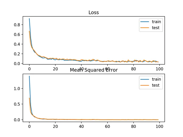
Line plots of Mean Absolute Error Loss and Mean Squared Error over Training Epochs