
There may be regression problems in which the target value has a spread of values and when predicting a large value, you may not want to punish a model as heavily as mean squared error.
Instead, you can first calculate the natural logarithm of each of the predicted values, then calculate the mean squared error. This is called the Mean Squared Logarithmic Error loss, or MSLE for short.
It has the effect of relaxing the punishing effect of large differences in large predicted values.
As a loss measure, it may be more appropriate when the model is predicting unscaled quantities directly. Nevertheless, we can demonstrate this loss function using our simple regression problem.
The model can be updated to use the ‘mean_squared_logarithmic_error‘ loss function and keep the same configuration for the output layer. We will also track the mean squared error as a metric when fitting the model so that we can use it as a measure of performance and plot the learning curve.
1 | model.compile(loss='mean_squared_logarithmic_error', optimizer=opt, metrics=['mse']) |
The complete example of using the MSLE loss function is listed below.

1 2 3 4 5 6 7 8 9 10 11 12 13 14 15 16 17 18 19 20 21 22 23 24 25 26 27 28 29 30 31 32 33 34 35 36 37 38 39 40 41 | # mlp for regression with msle loss function from sklearn.datasets import make_regression from sklearn.preprocessing import StandardScaler from keras.models import Sequential from keras.layers import Dense from keras.optimizers import SGD from matplotlib import pyplot # generate regression dataset X, y = make_regression(n_samples=1000, n_features=20, noise=0.1, random_state=1) # standardize dataset X = StandardScaler().fit_transform(X) y = StandardScaler().fit_transform(y.reshape(len(y),1))[:,0] # split into train and test n_train = 500 trainX, testX = X[:n_train, :], X[n_train:, :] trainy, testy = y[:n_train], y[n_train:] # define model model = Sequential() model.add(Dense(25, input_dim=20, activation='relu', kernel_initializer='he_uniform')) model.add(Dense(1, activation='linear')) opt = SGD(lr=0.01, momentum=0.9) model.compile(loss='mean_squared_logarithmic_error', optimizer=opt, metrics=['mse']) # fit model history = model.fit(trainX, trainy, validation_data=(testX, testy), epochs=100, verbose=0) # evaluate the model _, train_mse = model.evaluate(trainX, trainy, verbose=0) _, test_mse = model.evaluate(testX, testy, verbose=0) print('Train: %.3f, Test: %.3f' % (train_mse, test_mse)) # plot loss during training pyplot.subplot(211) pyplot.title('Loss') pyplot.plot(history.history['loss'], label='train') pyplot.plot(history.history['val_loss'], label='test') pyplot.legend() # plot mse during training pyplot.subplot(212) pyplot.title('Mean Squared Error') pyplot.plot(history.history['mean_squared_error'], label='train') pyplot.plot(history.history['val_mean_squared_error'], label='test') pyplot.legend() pyplot.show() |
Running the example first prints the mean squared error for the model on the train and test dataset.
Given the stochastic nature of the training algorithm, your specific results may vary. Try running the example a few times.
In this case, we can see that the model resulted in slightly worse MSE on both the training and test dataset. It may not be a good fit for this problem as the distribution of the target variable is a standard Gaussian.

1 | Train: 0.165, Test: 0.184 |
A line plot is also created showing the mean squared logistic error loss over the training epochs for both the train (blue) and test (orange) sets (top), and a similar plot for the mean squared error (bottom).
We can see that the MSLE converged well over the 100 epochs algorithm; it appears that the MSE may be showing signs of overfitting the problem, dropping fast and starting to rise from epoch 20 onwards.
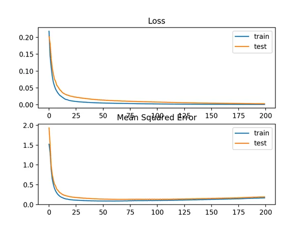
Line Plots of Mean Squared Logistic Error Loss and Mean Squared Error Over Training Epochs