
The Mean Squared Error, or MSE, loss is the default loss to use for regression problems.
Mathematically, it is the preferred loss function under the inference framework of maximum likelihood if the distribution of the target variable is Gaussian. It is the loss function to be evaluated first and only changed if you have a good reason.
Mean squared error is calculated as the average of the squared differences between the predicted and actual values. The result is always positive regardless of the sign of the predicted and actual values and a perfect value is 0.0. The squaring means that larger mistakes result in more error than smaller mistakes, meaning that the model is punished for making larger mistakes.
The mean squared error loss function can be used in Keras by specifying ‘mse‘ or ‘mean_squared_error‘ as the loss function when compiling the model.
1 | model.compile(loss='mean_squared_error') |
It is recommended that the output layer has one node for the target variable and the linear activation function is used.

1 | model.add(Dense(1, activation='linear')) |
A complete example of demonstrating an MLP on the described regression problem is listed below.

1 2 3 4 5 6 7 8 9 10 11 12 13 14 15 16 17 18 19 20 21 22 23 24 25 26 27 28 29 30 31 32 33 34 | # mlp for regression with mse loss function from sklearn.datasets import make_regression from sklearn.preprocessing import StandardScaler from keras.models import Sequential from keras.layers import Dense from keras.optimizers import SGD from matplotlib import pyplot # generate regression dataset X, y = make_regression(n_samples=1000, n_features=20, noise=0.1, random_state=1) # standardize dataset X = StandardScaler().fit_transform(X) y = StandardScaler().fit_transform(y.reshape(len(y),1))[:,0] # split into train and test n_train = 500 trainX, testX = X[:n_train, :], X[n_train:, :] trainy, testy = y[:n_train], y[n_train:] # define model model = Sequential() model.add(Dense(25, input_dim=20, activation='relu', kernel_initializer='he_uniform')) model.add(Dense(1, activation='linear')) opt = SGD(lr=0.01, momentum=0.9) model.compile(loss='mean_squared_error', optimizer=opt) # fit model history = model.fit(trainX, trainy, validation_data=(testX, testy), epochs=100, verbose=0) # evaluate the model train_mse = model.evaluate(trainX, trainy, verbose=0) test_mse = model.evaluate(testX, testy, verbose=0) print('Train: %.3f, Test: %.3f' % (train_mse, test_mse)) # plot loss during training pyplot.title('Loss / Mean Squared Error') pyplot.plot(history.history['loss'], label='train') pyplot.plot(history.history['val_loss'], label='test') pyplot.legend() pyplot.show() |
Running the example first prints the mean squared error for the model on the train and test datasets.
Given the stochastic nature of the training algorithm, your specific results may vary. Try running the example a few times.
In this case, we can see that the model learned the problem achieving zero error, at least to three decimal places.

1 | Train: 0.000, Test: 0.001 |
A line plot is also created showing the mean squared error loss over the training epochs for both the train (blue) and test (orange) sets.
We can see that the model converged reasonably quickly and both train and test performance remained equivalent. The performance and convergence behavior of the model suggest that mean squared error is a good match for a neural network learning this problem.
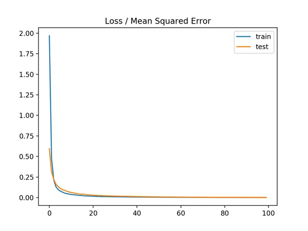
Line plot of Mean Squared Error Loss over Training Epochs When Optimizing the Mean Squared Error Loss Function