
Before we define a model, we need to contrive a problem that is appropriate for the weighted average ensemble.
In our problem, the training dataset is relatively small. Specifically, there is a 10:1 ratio of examples in the training dataset to the holdout dataset. This mimics a situation where we may have a vast number of unlabeled examples and a small number of labeled examples with which to train a model.
We will create 1,100 data points from the blobs problem. The model will be trained on the first 100 points and the remaining 1,000 will be held back in a test dataset, unavailable to the model.
The problem is a multi-class classification problem, and we will model it using a softmax activation function on the output layer. This means that the model will predict a vector with three elements with the probability that the sample belongs to each of the three classes. Therefore, we must one hot encode the class values before we split the rows into the train and test datasets. We can do this using the Keras to_categorical() function.
1 2 3 4 5 6 7 8 9 | # generate 2d classification dataset X, y = make_blobs(n_samples=1100, centers=3, n_features=2, cluster_std=2, random_state=2) # one hot encode output variable y = to_categorical(y) # split into train and test n_train = 100 trainX, testX = X[:n_train, :], X[n_train:, :] trainy, testy = y[:n_train], y[n_train:] print(trainX.shape, testX.shape) |
Next, we can define and compile the model.
The model will expect samples with two input variables. The model then has a single hidden layer with 25 nodes and a rectified linear activation function, then an output layer with three nodes to predict the probability of each of the three classes and a softmax activation function.
Because the problem is multi-class, we will use the categorical cross entropy loss function to optimize the model and the efficient Adam flavor of stochastic gradient descent.

1 2 3 4 5 | # define model model = Sequential() model.add(Dense(25, input_dim=2, activation='relu')) model.add(Dense(3, activation='softmax')) model.compile(loss='categorical_crossentropy', optimizer='adam', metrics=['accuracy']) |
The model is fit for 500 training epochs and we will evaluate the model each epoch on the test set, using the test set as a validation set.

1 2 | # fit model history = model.fit(trainX, trainy, validation_data=(testX, testy), epochs=500, verbose=0) |
At the end of the run, we will evaluate the performance of the model on the train and test sets.

1 2 3 4 | # evaluate the model _, train_acc = model.evaluate(trainX, trainy, verbose=0) _, test_acc = model.evaluate(testX, testy, verbose=0) print('Train: %.3f, Test: %.3f' % (train_acc, test_acc)) |
Then finally, we will plot learning curves of the model accuracy over each training epoch on both the training and validation datasets.

1 2 3 4 5 | # learning curves of model accuracy pyplot.plot(history.history['acc'], label='train') pyplot.plot(history.history['val_acc'], label='test') pyplot.legend() pyplot.show() |
Tying all of this together, the complete example is listed below.

1 2 3 4 5 6 7 8 9 10 11 12 13 14 15 16 17 18 19 20 21 22 23 24 25 26 27 28 29 30 31 | # develop an mlp for blobs dataset from sklearn.datasets.samples_generator import make_blobs from keras.utils import to_categorical from keras.models import Sequential from keras.layers import Dense from matplotlib import pyplot # generate 2d classification dataset X, y = make_blobs(n_samples=1100, centers=3, n_features=2, cluster_std=2, random_state=2) # one hot encode output variable y = to_categorical(y) # split into train and test n_train = 100 trainX, testX = X[:n_train, :], X[n_train:, :] trainy, testy = y[:n_train], y[n_train:] print(trainX.shape, testX.shape) # define model model = Sequential() model.add(Dense(25, input_dim=2, activation='relu')) model.add(Dense(3, activation='softmax')) model.compile(loss='categorical_crossentropy', optimizer='adam', metrics=['accuracy']) # fit model history = model.fit(trainX, trainy, validation_data=(testX, testy), epochs=500, verbose=0) # evaluate the model _, train_acc = model.evaluate(trainX, trainy, verbose=0) _, test_acc = model.evaluate(testX, testy, verbose=0) print('Train: %.3f, Test: %.3f' % (train_acc, test_acc)) # learning curves of model accuracy pyplot.plot(history.history['acc'], label='train') pyplot.plot(history.history['val_acc'], label='test') pyplot.legend() pyplot.show() |
Running the example first prints the shape of each dataset for confirmation, then the performance of the final model on the train and test datasets.
Your specific results will vary (by design!) given the high variance nature of the model.
In this case, we can see that the model achieved about 87% accuracy on the training dataset, which we know is optimistic, and about 81% on the test dataset, which we would expect to be more realistic.

1 2 | (100, 2) (1000, 2) Train: 0.870, Test: 0.814 |
A line plot is also created showing the learning curves for the model accuracy on the train and test sets over each training epoch.
We can see that training accuracy is more optimistic over most of the run as we also noted with the final scores.
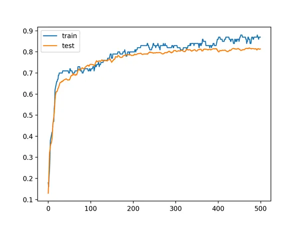
Line Plot Learning Curves of Model Accuracy on Train and Test Dataset over Each Training Epoch
Now that we have identified that the model is a good candidate for developing an ensemble, we can next look at developing a simple model averaging ensemble.