
A modeling averaging ensemble combines the prediction from each model equally and often results in better performance on average than a given single model.
Sometimes there are very good models that we wish to contribute more to an ensemble prediction, and perhaps less skillful models that may be useful but should contribute less to an ensemble prediction. A weighted average ensemble is an approach that allows multiple models to contribute to a prediction in proportion to their trust or estimated performance.
In this tutorial, you will discover how to develop a weighted average ensemble of deep learning neural network models in Python with Keras.
After completing this tutorial, you will know:
· Model averaging ensembles are limited because they require that each ensemble member contribute equally to predictions.
· Weighted average ensembles allow the contribution of each ensemble member to a prediction to be weighted proportionally to the trust or performance of the member on a holdout dataset.
· How to implement a weighted average ensemble in Keras and compare results to a model averaging ensemble and standalone models.
Let’s get started.
We will use a small multi-class classification problem as the basis to demonstrate the weighted averaging ensemble.
The scikit-learn class provides the make_blobs() function that can be used to create a multi-class classification problem with the prescribed number of samples, input variables, classes, and variance of samples within a class.
The problem has two input variables (to represent the x and y coordinates of the points) and a standard deviation of 2.0 for points within each group. We will use the same random state (seed for the pseudorandom number generator) to ensure that we always get the same data points.
1 2 | # generate 2d classification dataset X, y = make_blobs(n_samples=1000, centers=3, n_features=2, cluster_std=2, random_state=2) |
The results are the input and output elements of a dataset that we can model.
In order to get a feeling for the complexity of the problem, we can plot each point on a two-dimensional scatter plot and color each point by class value.
The complete example is listed below.
1 2 3 4 5 6 7 8 9 10 11 12 13 14 | # scatter plot of blobs dataset from sklearn.datasets.samples_generator import make_blobs from matplotlib import pyplot from pandas import DataFrame # generate 2d classification dataset X, y = make_blobs(n_samples=1000, centers=3, n_features=2, cluster_std=2, random_state=2) # scatter plot, dots colored by class value df = DataFrame(dict(x=X[:,0], y=X[:,1], label=y)) colors = {0:'red', 1:'blue', 2:'green'} fig, ax = pyplot.subplots() grouped = df.groupby('label') for key, group in grouped: group.plot(ax=ax, kind='scatter', x='x', y='y', label=key, color=colors[key]) pyplot.show() |
Running the example creates a scatter plot of the entire dataset. We can see that the standard deviation of 2.0 means that the classes are not linearly separable (separable by a line) causing many ambiguous points.
This is desirable as it means that the problem is non-trivial and will allow a neural network model to find many different “good enough” candidate solutions resulting in a high variance.
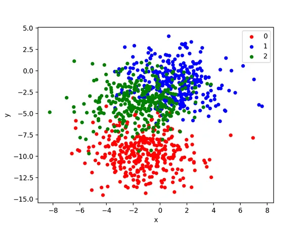
Scatter Plot of Blobs Dataset With Three Classes and Points Colored by Class Value