
This section assumes that you are using the TensorFlow backend with Keras. If this is not the case, you can skip this section.
In the cases of using the tanh activation function, we know the network has more than enough capacity to learn the problem, but the increase in layers has prevented it from doing so.
It is hard to diagnose a vanishing gradient as a cause for bad performance. One possible signal is to review the average size of the gradient per layer per training epoch.
We would expect layers closer to the output to have a larger average gradient than those layers closer to the input.
Keras provides the TensorBoard callback that can be used to log properties of the model during training such as the average gradient per layer. These statistics can then be reviewed using the TensorBoard interface that is provided with TensorFlow.
We can configure this callback to record the average gradient per-layer per-training epoch, then ensure the callback is used as part of training the model.
1 2 3 4 | # prepare callback tb = TensorBoard(histogram_freq=1, write_grads=True) # fit model model.fit(trainX, trainy, validation_data=(testX, testy), epochs=500, verbose=0, callbacks=[tb]) |
We can use this callback to first investigate the dynamics of the gradients in the deep model fit using the hyperbolic tangent activation function, then later compare the dynamics to the same model fit using the rectified linear activation function.
First, the complete example of the deep MLP model using tanh and the TensorBoard callback is listed below.

1 2 3 4 5 6 7 8 9 10 11 12 13 14 15 16 17 18 19 20 21 22 23 24 25 26 27 28 29 30 31 32 | # deeper mlp for the two circles classification problem with callback from sklearn.datasets import make_circles from sklearn.preprocessing import MinMaxScaler from keras.layers import Dense from keras.models import Sequential from keras.optimizers import SGD from keras.initializers import RandomUniform from keras.callbacks import TensorBoard # generate 2d classification dataset X, y = make_circles(n_samples=1000, noise=0.1, random_state=1) scaler = MinMaxScaler(feature_range=(-1, 1)) X = scaler.fit_transform(X) # split into train and test n_train = 500 trainX, testX = X[:n_train, :], X[n_train:, :] trainy, testy = y[:n_train], y[n_train:] # define model init = RandomUniform(minval=0, maxval=1) model = Sequential() model.add(Dense(5, input_dim=2, activation='tanh', kernel_initializer=init)) model.add(Dense(5, activation='tanh', kernel_initializer=init)) model.add(Dense(5, activation='tanh', kernel_initializer=init)) model.add(Dense(5, activation='tanh', kernel_initializer=init)) model.add(Dense(5, activation='tanh', kernel_initializer=init)) model.add(Dense(1, activation='sigmoid', kernel_initializer=init)) # compile model opt = SGD(lr=0.01, momentum=0.9) model.compile(loss='binary_crossentropy', optimizer=opt, metrics=['accuracy']) # prepare callback tb = TensorBoard(histogram_freq=1, write_grads=True) # fit model model.fit(trainX, trainy, validation_data=(testX, testy), epochs=500, verbose=0, callbacks=[tb]) |
Running the example creates a new “logs/” subdirectory with a file containing the statistics recorded by the callback during training.
We can review the statistics in the TensorBoard web interface. The interface can be started from the command line, requiring that you specify the full path to your logs directory.
For example, if you run the code in a “/code” directory, then the full path to the logs directory will be “/code/logs/“.
Below is the command to start the TensorBoard interface to be executed on your command line (command prompt). Be sure to change the path to your logs directory.

1 | python -m tensorboard.main --logdir=/code/logs/ |
Next, open your web browser and enter the following URL:
· http://localhost:6006
If all went well, you will see the TensorBoard web interface.
Plots of the average gradient per layer per training epoch can be reviewed under the “Distributions” and “Histograms” tabs of the interface. The plots can be filtered to only show the gradients for the Dense layers, excluding the bias, using the search filter “kernel_0_grad“.
I have provided a copy of the plots below, although your specific results may vary given the stochastic nature of the learning algorithm.
First, line plots are created for each of the 6 layers (5 hidden, 1 output). The names of the plots indicate the layer, where “dense_1” indicates the hidden layer after the input layer and “dense_6” represents the output layer.
We can see that the output layer has a lot of activity over the entire run, with average gradients per epoch at around 0.05 to 0.1. We can also see some activity in the first hidden layer with a similar range. Therefore, gradients are getting through to the first hidden layer, but the last layer and last hidden layer is seeing most of the activity.

TensorBoard Line Plots of Average Gradients Per Layer for Deep MLP With Tanh
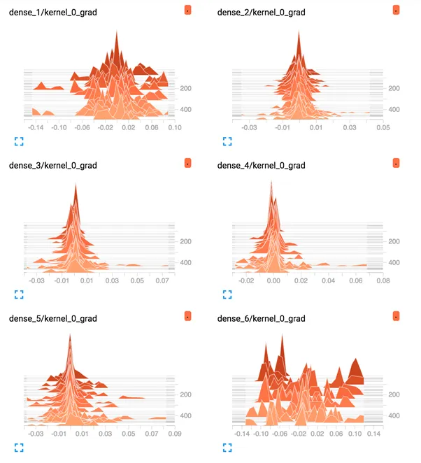
TensorBoard Density Plots of Average Gradients Per Layer for Deep MLP With Tanh
We can collect the same information from the deep MLP with the ReLU activation function.
The complete example is listed below.
1 2 3 4 5 6 7 8 9 10 11 12 13 14 15 16 17 18 19 20 21 22 23 24 25 26 27 28 29 30 | # deeper mlp with relu for the two circles classification problem with callback from sklearn.datasets import make_circles from sklearn.preprocessing import MinMaxScaler from keras.layers import Dense from keras.models import Sequential from keras.optimizers import SGD from keras.callbacks import TensorBoard # generate 2d classification dataset X, y = make_circles(n_samples=1000, noise=0.1, random_state=1) scaler = MinMaxScaler(feature_range=(-1, 1)) X = scaler.fit_transform(X) # split into train and test n_train = 500 trainX, testX = X[:n_train, :], X[n_train:, :] trainy, testy = y[:n_train], y[n_train:] # define model model = Sequential() model.add(Dense(5, input_dim=2, activation='relu', kernel_initializer='he_uniform')) model.add(Dense(5, activation='relu', kernel_initializer='he_uniform')) model.add(Dense(5, activation='relu', kernel_initializer='he_uniform')) model.add(Dense(5, activation='relu', kernel_initializer='he_uniform')) model.add(Dense(5, activation='relu', kernel_initializer='he_uniform')) model.add(Dense(1, activation='sigmoid')) # compile model opt = SGD(lr=0.01, momentum=0.9) model.compile(loss='binary_crossentropy', optimizer=opt, metrics=['accuracy']) # prepare callback tb = TensorBoard(histogram_freq=1, write_grads=True) # fit model model.fit(trainX, trainy, validation_data=(testX, testy), epochs=500, verbose=0, callbacks=[tb]) |
The TensorBoard interface can be confusing if you are new to it.
To keep things simple, delete the “logs” subdirectory prior to running this second example.
Once run, you can start the TensorBoard interface the same way and access it through your web browser.
The plots of the average gradient per layer per training epoch show a different story as compared to the gradients for the deep model with tanh.
We can see that the first hidden layer sees more gradients, more consistently with larger spread, perhaps 0.2 to 0.4, as opposed to 0.05 and 0.1 seen with tanh. We can also see that the middle hidden layers see large gradients.

TensorBoard Line Plots of Average Gradients Per Layer for Deep MLP With ReLU
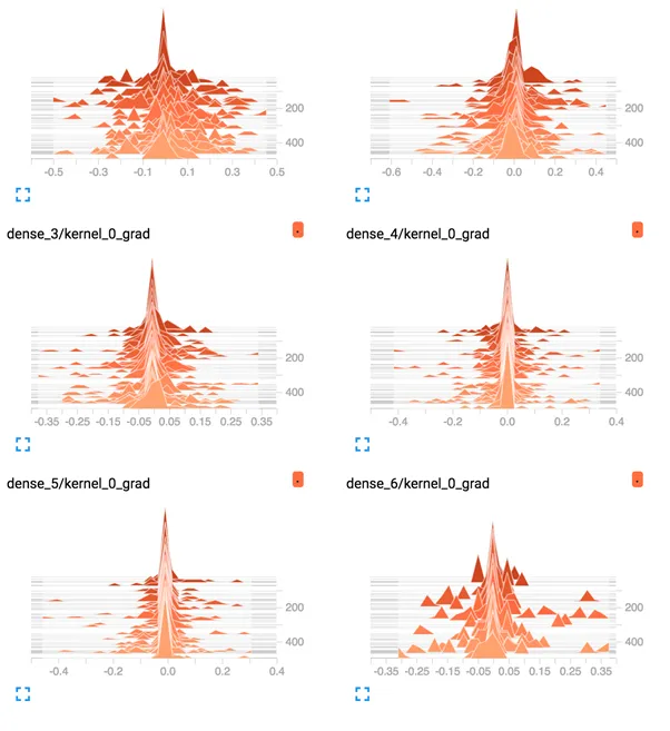
TensorBoard Density Plots of Average Gradients Per Layer for Deep MLP With ReLU
The ReLU activation function is allowing more gradient to flow backward through the model during training, and this may be the cause for improved performance