
The rectified linear activation function has supplanted the hyperbolic tangent activation function as the new preferred default when developing Multilayer Perceptron networks, as well as other network types like CNNs.
This is because the activation function looks and acts like a linear function, making it easier to train and less likely to saturate, but is, in fact, a nonlinear function, forcing negative inputs to the value 0. It is claimed as one possible approach to addressing the vanishing gradients problem when training deeper models.
When using the rectified linear activation function (or ReLU for short), it is good practice to use the He weight initialization scheme. We can define the MLP with five hidden layers using ReLU and He initialization, listed below.
1 2 3 4 5 6 7 8 | # define model model = Sequential() model.add(Dense(5, input_dim=2, activation='relu', kernel_initializer='he_uniform')) model.add(Dense(5, activation='relu', kernel_initializer='he_uniform')) model.add(Dense(5, activation='relu', kernel_initializer='he_uniform')) model.add(Dense(5, activation='relu', kernel_initializer='he_uniform')) model.add(Dense(5, activation='relu', kernel_initializer='he_uniform')) model.add(Dense(1, activation='sigmoid')) |
Tying this together, the complete code example is listed below.

1 2 3 4 5 6 7 8 9 10 11 12 13 14 15 16 17 18 19 20 21 22 23 24 25 26 27 28 29 30 31 32 33 34 35 36 37 38 | # deeper mlp with relu for the two circles classification problem from sklearn.datasets import make_circles from sklearn.preprocessing import MinMaxScaler from keras.layers import Dense from keras.models import Sequential from keras.optimizers import SGD from keras.initializers import RandomUniform from matplotlib import pyplot # generate 2d classification dataset X, y = make_circles(n_samples=1000, noise=0.1, random_state=1) scaler = MinMaxScaler(feature_range=(-1, 1)) X = scaler.fit_transform(X) # split into train and test n_train = 500 trainX, testX = X[:n_train, :], X[n_train:, :] trainy, testy = y[:n_train], y[n_train:] # define model model = Sequential() model.add(Dense(5, input_dim=2, activation='relu', kernel_initializer='he_uniform')) model.add(Dense(5, activation='relu', kernel_initializer='he_uniform')) model.add(Dense(5, activation='relu', kernel_initializer='he_uniform')) model.add(Dense(5, activation='relu', kernel_initializer='he_uniform')) model.add(Dense(5, activation='relu', kernel_initializer='he_uniform')) model.add(Dense(1, activation='sigmoid')) # compile model opt = SGD(lr=0.01, momentum=0.9) model.compile(loss='binary_crossentropy', optimizer=opt, metrics=['accuracy']) # fit model history = model.fit(trainX, trainy, validation_data=(testX, testy), epochs=500, verbose=0) # evaluate the model _, train_acc = model.evaluate(trainX, trainy, verbose=0) _, test_acc = model.evaluate(testX, testy, verbose=0) print('Train: %.3f, Test: %.3f' % (train_acc, test_acc)) # plot training history pyplot.plot(history.history['acc'], label='train') pyplot.plot(history.history['val_acc'], label='test') pyplot.legend() pyplot.show() |
Running the example prints the performance of the model on the train and test datasets.
Your specific results may vary given the stochastic nature of the learning algorithm. Consider running the example a few times.
In this case, we can see that this small change has allowed the model to learn the problem, achieving about 84% accuracy on both datasets, outperforming the single layer model using the tanh activation function.

1 | Train: 0.836, Test: 0.840 |
A line plot of model accuracy on the train and test sets over training epochs is also created. The plot shows quite different dynamics to what we have seen so far.
The model appears to rapidly learn the problem, converging on a solution in about 100 epochs.
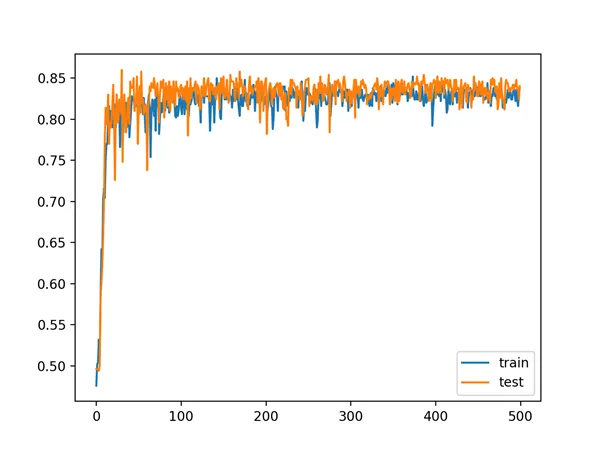
Line Plot of Train and Test Set Accuracy of Over Training Epochs for Deep MLP with ReLU in the Two Circles Problem
Use of the ReLU activation function has allowed us to fit a much deeper model for this simple problem, but this capability does not extend infinitely. For example, increasing the number of layers results in slower learning to a point at about 20 layers where the model is no longer capable of learning the problem, at least with the chosen configuration.
For example, below is a line plot of train and test accuracy of the same model with 15 hidden layers that shows that it is still capable of learning the problem.
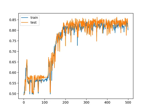
Line Plot of Train and Test Set Accuracy of Over Training Epochs for Deep MLP with ReLU with 15 Hidden Layers
Below is a line plot of train and test accuracy over epochs with the same model with 20 layers, showing that the configuration is no longer capable of learning the problem.

Line Plot of Train and Test Set Accuracy of Over Training Epochs for Deep MLP with ReLU with 20 Hidden Layers
Although use of the ReLU worked, we cannot be confident that use of the tanh function failed because of vanishing gradients and ReLU succeed because it overcame this problem.