How to Fix Vanishing Gradients Using the Rectified Linear Activation Function

The vanishing gradients problem is one example of unstable behavior that you may encounter when training a deep neural network.

It describes the situation where a deep multilayer feed-forward network or a recurrent neural network is unable to propagate useful gradient information from the output end of the model back to the layers near the input end of the model.

The result is the general inability of models with many layers to learn on a given dataset or to prematurely converge to a poor solution.

Many fixes and workarounds have been proposed and investigated, such as alternate weight initialization schemes, unsupervised pre-training, layer-wise training, and variations on gradient descent. Perhaps the most common change is the use of the rectified linear activation function that has become the new default, instead of the hyperbolic tangent activation function that was the default through the late 1990s and 2000s.

In this tutorial, you will discover how to diagnose a vanishing gradient problem when training a neural network model and how to fix it using an alternate activation function and weight initialization scheme.

After completing this tutorial, you will know:

·         The vanishing gradients problem limits the development of deep neural networks with classically popular activation functions such as the hyperbolic tangent.

·         How to fix a deep neural network Multilayer Perceptron for classification using ReLU and He weight initialization.

·         How to use TensorBoard to diagnose a vanishing gradient problem and confirm the impact of ReLU to improve the flow of gradients through the model.

Let’s get started.

Two Circles Binary Classification Problem

As the basis for our exploration, we will use a very simple two-class or binary classification problem.

The scikit-learn class provides the make_circles() function that can be used to create a binary classification problem with the prescribed number of samples and statistical noise.

Each example has two input variables that define the x and y coordinates of the point on a two-dimensional plane. The points are arranged in two concentric circles (they have the same center) for the two classes.

The number of points in the dataset is specified by a parameter, half of which will be drawn from each circle. Gaussian noise can be added when sampling the points via the “noise” argument that defines the standard deviation of the noise, where 0.0 indicates no noise or points drawn exactly from the circles. The seed for the pseudorandom number generator can be specified via the “random_state” argument that allows the exact same points to be sampled each time the function is called.

The example below generates 1,000 examples from the two circles with noise and a value of 1 to seed the pseudorandom number generator.

We can create a graph of the dataset, plotting the x and y coordinates of the input variables (X) and coloring each point by the class value (0 or 1).

The complete example is listed below.

Running the example creates a plot showing the 1,000 generated data points with the class value of each point used to color each point.

We can see points for class 0 are blue and represent the outer circle, and points for class 1 are orange and represent the inner circle.

The statistical noise of the generated samples means that there is some overlap of points between the two circles, adding some ambiguity to the problem, making it non-trivial. This is desirable as a neural network may choose one of among many possible solutions to classify the points between the two circles and always make some errors.

Scatter Plot of Circles Dataset With Points Colored By Class Value

Now that we have defined a problem as the basis for our exploration, we can look at developing a model to address it.

Multilayer Perceptron Model for Two Circles Problem

We can develop a Multilayer Perceptron model to address the two circles problem.

This will be a simple feed-forward neural network model, designed as we were taught in the late 1990s and early 2000s.

First, we will generate 1,000 data points from the two circles problem and rescale the inputs to the range [-1, 1]. The data is almost already in this range, but we will make sure.

Normally, we would prepare the data scaling using a training dataset and apply it to a test dataset. To keep things simple in this tutorial, we will scale all of the data together before splitting it into train and test sets.

Next, we will split the data into train and test sets.

Half of the data will be used for training and the remaining 500 examples will be used as the test set. In this tutorial, the test set will also serve as the validation dataset so we can get an idea of how the model performs on the holdout set during training.

Next, we will define the model.

The model will have an input layer with two inputs, for the two variables in the dataset, one hidden layer with five nodes, and an output layer with one node used to predict the class probability. The hidden layer will use the hyperbolic tangent activation function (tanh) and the output layer will use the logistic activation function (sigmoid) to predict class 0 or class 1 or something in between.

Using the hyperbolic tangent activation function in hidden layers was the best practice in the 1990s and 2000s, performing generally better than the logistic function when used in the hidden layer. It was also good practice to initialize the network weights to small random values from a uniform distribution. Here, we will initialize weights randomly from the range [0.0, 1.0].

The model uses the binary cross entropy loss function and is optimized using stochastic gradient descent with a learning rate of 0.01 and a large momentum of 0.9.

The model is trained for 500 training epochs and the test dataset is evaluated at the end of each epoch along with the training dataset.

After the model is fit, it is evaluated on both the train and test dataset and the accuracy scores are displayed.

Finally, the accuracy of the model during each step of training is graphed as a line plot, showing the dynamics of the model as it learned the problem.

Tying all of this together, the complete example is listed below.

Running the example fits the model in just a few seconds.

The model performance on the train and test sets is calculated and displayed. Your specific results may vary given the stochastic nature of the learning algorithm. Consider running the example a few times.

We can see that in this case, the model learned the problem well, achieving an accuracy of about 81.6% on both the train and test datasets.

A line plot of model accuracy on the train and test sets is created, showing the change in performance over all 500 training epochs.

The plot suggests, for this run, that the performance begins to slow around epoch 300 at about 80% accuracy for both the train and test sets.

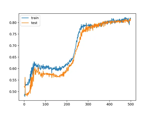
Line Plot of Train and Test Set Accuracy Over Training Epochs for MLP in the Two Circles Problem

Now that we have seen how to develop a classical MLP using the tanh activation function for the two circles problem, we can look at modifying the model to have many more hidden layers.

Deeper MLP Model for Two Circles Problem

Traditionally, developing deep Multilayer Perceptron models was challenging.

Deep models using the hyperbolic tangent activation function do not train easily, and much of this poor performance is blamed on the vanishing gradient problem.

We can attempt to investigate this using the MLP model developed in the previous section.

The number of hidden layers can be increased from 1 to 5; for example:

We can then re-run the example and review the results.

The complete example of the deeper MLP is listed below.

Running the example first prints the performance of the fit model on the train and test datasets.

Your specific results may vary given the stochastic nature of the learning algorithm. Consider running the example a few times.

In this case, we can see that performance is quite poor on both the train and test sets achieving around 50% accuracy. This suggests that the model as configured could not learn the problem nor generalize a solution.

The line plots of model accuracy on the train and test sets during training tell a similar story. We can see that performance is bad and actually gets worse as training progresses.

Line Plot of Train and Test Set Accuracy of Over Training Epochs for Deep MLP in the Two Circles Problem