The Bobillier Constructions

The Hartmann construction provides one graphical method of finding the conjugate point and the radius of curvature of the path of a moving point, but it requires knowledge of the curvature of the fixed and moving centrodes. It would be desirable to have graphical methods of obtaining the inflection circle and the conjugate of a given point without requiring the curvature of the centrodes. Such graphical solutions are presented in this section and are called the Bobillier constructions.

To understand these constructions, consider the inflection circle and the centrode normal Nand centrode tangent T shown in Fig. 4.27. Let us select any two points A and B of the moving body which are not on a straight line through P. Now, by using the Euler-Savary equation, we can find the two corresponding conjugate points A' and B'. The intersection of the lines AB and A' B' is labelled Q. Then, the straight line drawn through P and Q is called the collineation axis. This axis applies only to the two lines AA' and BB' and so is said to belong to these two rays; also, the point Q will be located differently on the collineation axis if another set of points A and B is chosen on the same rays. Nevertheless, there is a unique relationship between the collineation axis and the two rays used to define it. This relationship is expressed in Bobillier 's theorem, which states that the angle from the centrode tangent to one of these rays is the negative of the angle from the collineation axis to the other ray

In applying the Euler-Savary equation to a planar mechanism, we can usually find two pairs of conjugate points by inspection, and from these we wish to determine the inflection circle graphically. For example, a four-bar linkage with a crank 02A and a follower 04B has A and O2 as one set of conjugate points and Band 04 as the other, when we are interested in the motion of the coupler relative to the frame. Given these two pairs of conjugate points, how do we use the Bobillier theorem to find the inflection circle?

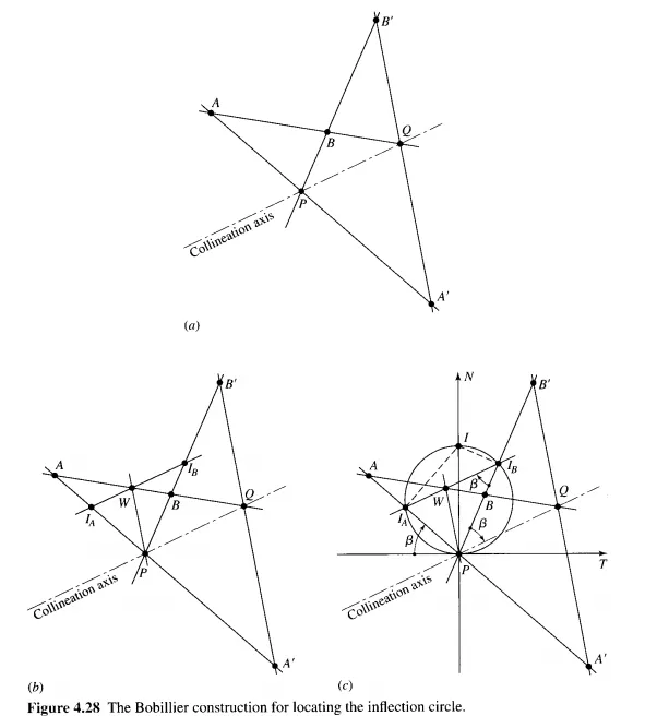
In Fig. 4.28a, let A and A' and Band B' represent the known pairs of conjugate points. Rays constructed through each pair intersect at P, the instant center of velocity, giving one point on the inflection circle. Point Q is located next by the intersection of a ray through A and B with a ray through A' and B'. Then the collineation axis can be drawn as the line PQ.

The next step is shown in Fig. 4.28b. Drawing a straight line through P parallel to A' B', we identify the point W as the intersection of this line with the line AB. Now, through W we draw a second line parallel to the collineation axis. This line intersects AA' at IA and B B' at Is, the two additional points on the inflection circle for which we are searching.

We could now construct the circle through the three points I A, Is, and P, but there is an easier way. Remembering that a triangle inscribed in a semicircle is a right triangle having the diameter as its hypotenuse, we erect a perpendicular to A P at I A and another perpendicular to B P at Is. The intersection of these two perpendiculars gives point I, the inflection pole, as shown in Fig. 4.28c. Because P I is the diameter, the inflection circle, the centrode normal N, and the centrode tangent T can all be easily constructed.

To show that this construction satisfies the Bobillier theorem, note that the arc from P to I A is inscribed by the angle that lAP makes with the centrode tangent. But this same arc is also inscribed by the angle PIsIA. Therefore these two angles are equal. But the line IslA was originally constructed parallel to the collineation axis. Therefore, the line PIs also makes the same angle f3 with the collineation axis.

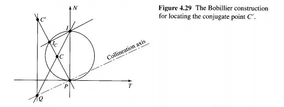
Our final problem is to learn how to use the Bobillier theorem to find the conjugate of another arbitrary point, say C, when the inflection circle is given. In Fig. 4.29 we join C

with the instant center P and locate the intersection point Ie with the inflection circle. This ray serves as one of the two necessary to locate the collineation axis. For the other we may as well use the centrode normal, because I and its conjugate point 1', at infinity, are both known. For these two rays the collineation axis is a line through P parallel to the line Ie I, as we learned in Fig. 4.28c. The balance of the construction is similar to that of Fig. 4.27. Point Q is located by the intersection of a line through I and C with the collineation axis. Then a line through Q and l' at infinity intersects the ray PC at C', the conjugate point for C.