What is a Lognormal Distribution?
A lognormal (log-normal or Galton) distribution is a probability distribution with a normally distributed logarithm. A random variable is lognormally distributed if its logarithm is normally distributed.
Skewed distributions with low mean values, large variance, and all-positive values often fit this type of distribution. Values must be positive as log(x) exists only for positive values of x.
The probability density function is defined by the mean μ and standard deviation, σ:
The shape of the lognormal distribution is defined by three parameters:
· σ, the shape parameter. Also the standard deviation for the lognormal, this affects the general shape of the distribution. Usually, these parameters are known from historical data. Sometimes, you might be able to estimate it with current data. The shape parameter doesn’t change the location or height of the graph; it just affects the overall shape.
· m, the scale parameter (this is also the median). This parameter shrinks or stretches the graph.
· Θ (or μ), the location parameter, which tells you where on the x-axis the graph is located.
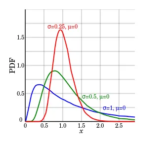
The standard lognormal distribution has a location parameter of 0 and a scale parameter of 1 (shown in blue in the image below). If Θ = 0, the distribution is called a 2-parameter lognormal distribution.

A few examples of lognormal density functions.
The most commonly used (and the most familiar) distribution in science is the normal distribution. The familiar “bell curve” models many natural phenomenon, from the simple (weights or heights) to the more complex. For example, the following phenomenon can all be modeled with a lognormal distribution:
· Milk production by cows.
· Lives of industrial units with failure modes that are characterized by fatigue-stress.
· Amounts of rainfall.
· Size distributions of rainfall droplets.
· The volume of gas in a petroleum reserve.
Many more phenomenon can be modeled with the lognormal distribution, such as the length of latent periods of infectious disease or species abundance1.
Historically, the lognormal distribution has been called many names, including:
· The Galton or Galton’s distribution (after the Victorian statistician Francis Galton).
· Galton-McAlister distribution (McAlister was another Victorian statistician who published a description of the distribution with Galton).
· Gibrat distribution, after the 20th century French economist who showed that the logarithms of certain economic variables (like factory distribution by number of workers) followed a normal distribution.
· Cobb-Douglas distribution (after 20th century economists Charles Cobb and Paul Douglas). This term is used exclusively in economics, where it’s applied to production data.