Different Mesh Refinement Metrics

Studying convergence requires choosing an appropriate mesh refinement metric. This metric can be either local or global. That is, the metric can be defined at one location in the model or as the integral of the fields over the entire model space. An example of a local metric is the displacement or stress at a point within a structural analysis. An example of a global metric is the integral of the strain energy density over all domains. Both the stresses and the strain are computed based upon the gradient of the solution and the displacement field. Gradients of the solution are always computed to one order lower polynomial approximation.

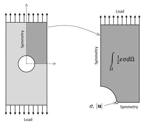
A simple finite element model of a loaded plate with a hole. Symmetry is used to reduce the model size, and several different metrics can be defined to study mesh refinement.

While choosing a metric, it is important to remember that different metrics will have different convergence behavior. This is illustrated in the figure below, showing different meshes being used to solve the same FEA model. These meshes differ in terms of the element size and are compared in terms of the number of degrees of freedom (DOF) within the model. The DOF is related to the number of nodes, the computational points that define the shape of each finite element. The computational resources required to solve an FEA model are directly related to the number of DOF.

From the figure below, it appears as if certain metrics converge faster than others, but it is important to keep in mind that the rate of mesh convergence for a particular problem statement is dependent upon which mesh refinement technique is used.

Convergence of a global metric (top), a local metric based upon the solution field (center), and a local metric based upon the gradient of the solution (bottom) with 1% error bars compared to the most refined solution. The same meshes were used for the three cases.

Different Mesh Refinement Techniques

When it comes to mesh refinement, there is a suite of techniques that are commonly used. An experienced user of FEA software should be familiar with each of these techniques and the tradeoffs between them.

Reducing the Element Size

Reducing the element size is the easiest mesh refinement strategy, with element sizes reduced throughout the modeling domains. This approach is attractive due to its simplicity, but the drawback is that there is no preferential mesh refinement in regions where a locally finer mesh may be needed.

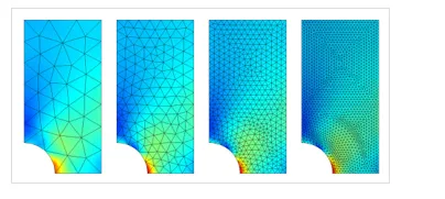
The stresses in a plate with a hole, solved with different element sizes.

Increasing the Element Order

Increasing the element order is advantageous in the sense that no remeshing is needed; the same mesh can be used, but with different element orders. Remeshing can be time consuming for complex 3D geometries or the mesh may come from an external source and cannot be altered. The disadvantage to this technique is that the computational requirements increase faster than with other mesh refinement techniques.

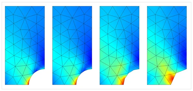
The same finite element mesh, but solved with different element orders.