What is the difference between serendipity family elements and isoparametric elements in finite element analysis?

In the Finite Element Method we use several types of elements. These elements can be classified based upon the dimensionality ( ID, II D and III D Elements) or on the order of the element ( Lower order and Higher order elements).

The lower order elements are also referred to as Linear elements as the displacement models and hence the shape functions are linear.

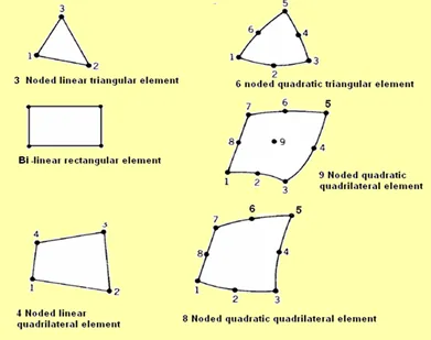
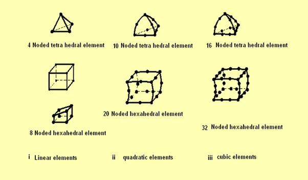
Among higher order elements we have quadratic and cubic elements where the variation of the field variables expressed in terms of shape functions are respectively quadratic and cubic. The figures shown below show some 2D and 3D linear and quadratic elements.

Now in the 2D elements there are both 9 noded and 8 noded quadratic quadrilateral elements. Higher order elements in 2D and 3D with no internal nodes are referred to as Serendipity elements. It can be noted that the 6 noded triangular and 8 noded quadrilateral elements have no nodes inside the element, ie no interior nodes. Advantage of removing one one node in a 9 noded quadrilateral element with two variables per node is that the size of the stiffness matrix reduces from 18 x 18 to 16 x 16 and consider a problem where we have about 50,000 elements. There is considerable reduction in the size of the global stiffness matrix and hence the computation time for solving.

So in short Serendipity elements are higher order elements in 2D and 3D with no internal nodes which lead to considerable saving in storage space and computation time.

Now coming to isoparametric elements, it can be seen that higher order elements in 2D and 3D may have curved sides. Because of this we cannot derive the shape functions easily. Hence we map these elements into natural coordinates space where the absolute coordinates of each element does not exceed unity (one). When mapping a curved side element it becomes a square of size 2 x 2. We can then use some method of deriving shape functions keeping in mind the properties of shape functions. (Has a value one at the node it is associated with and a value zero at all other nodes)

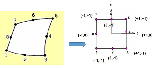
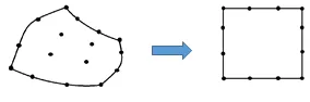
The figures shown above shows how a curved side element in Cartesian coordinates becomes a regular square shaped element when mapped to natural coordinate space.

Such elements are called isoparametric elements when the same shape functions are used for the field variable approximation as well as the for the geometric transformation from Cartesian space to natural coordinate space.

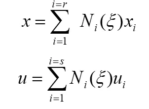
When r=s ie the same order polynomial is used for both geometric transformation as in first equation above and field variable approximation as in the second equation then we call the elements as Isoparametric elements.

There is much more to this but I think this explains the difference between Serendipity elements and Isoparametric elements. :)