Force and Compliance Controls

A class of simple tasks may need only trajectory control where the robot end-effecter is moved merely along a prescribed time trajectory. However, a number of complex tasks, including assembly of parts, manipulation of tools, and walking on a terrain, entail the control of physical interactions and mechanical contacts with the environment. Achieving a task goal often requires the robot to comply with the environment, react to the force acting on the end-effecter, or adapt its motion to uncertainties of the environment. Strategies are needed for performing those tasks.

 Force and compliance controls are fundamental task strategies for performing a class of tasks entailing the accommodation of mechanical interactions in the face of environmental uncertainties. In this chapter we will first present hybrid position/force control: a basic principle of strategic task planning for dealing with geometric constraints imposed by the task environment. An alternative approach to accommodating interactions will also be presented based on compliance or stiffness control. Characteristics of task compliances and force feedback laws will be analyzed and applied to various tasks.

Hybrid Position/Force Control

Principle

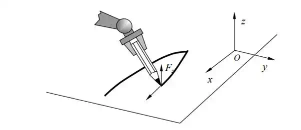
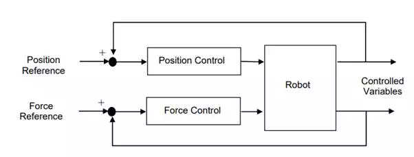
To begin with let us consider a daily task. Figure 9.1.1 illustrates a robot drawing a line with a pencil on a sheet of paper. Although we humans can perform this type of task without considering any detail of hand control, the robot needs specific control commands and an effective control strategy. To draw a letter, “A”, for example, we first conceive a trajectory of the pencil tip, and command the hand to follow the conceived trajectory. At the same time we accommodate the pressure with which the pencil is contacting the sheet of paper. Let o-xyz be a coordinate system with the z-axis perpendicular to the sheet of paper. Along the x and y axes, we provide positional commands to the hand control system. Along the z-axis, on the other hand, we specify a force to apply. In other words, controlled variables are different between the horizontal and vertical directions. The controlled variable of the former is x and y coordinates, i.e. a position, while the latter controlled variable is a force in the z direction. Namely, two types of control loops are combined in the hand control system, as illustrated.

Robot drawing a line with a pencil on a sheet of paper

Position and force control loops

The above example is one of the simplest tasks illustrating the need for integrating different control loops in such a way that the control mode is consistent with the geometric constraint imposed to the robot system. As the geometric constraint becomes more complex and the task objective is more involved, an intuitive method may not suffice. In the following we will obtain a general principle that will help us find proper control modes consistent with both geometric constraints and task objectives. Let us consider the following six-dimensional task to derive a basic principle behind our heuristics and empiricism.

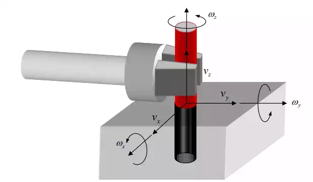
Shown below is a task to pull up a peg from a hole. We assume that the peg can move in the vertical direction without friction when sliding in the hole. We also assume that the task process is quasi-static in that any inertial force is negligibly small. A coordinate system O-xyz, referred to as C-frame, is attached to the task space, as shown in the figure. The problem is to find a proper control mode for each of the axes: three translational and three rotational axes.

Pulling up a peg from a hole

The key question is how to assign a control mode, position control or force control, to each of the axes in the C-frame in such a way that the control action may not conflict with the geometric constraints and physics. M. Mason addressed this issue in his seminal work on hybrid position/force control. He called conditions dictated by physics Natural Constraints, and conditions determined by task goals and objectives Artificial Constraints. Table 9.1.1 summarizes these conditions.

it is clear that the peg cannot be moved in the x and y directions due to the geometric constraint. Therefore, the velocities in these directions must be zero: . Likewise, the peg cannot be rotated about the x and y axes. Therefore, the angular velocities are zero: . These conditions constitute the natural constraints in the kinematic domain. The remaining directions are linear and angular z axes. Velocities along these two directions can be assigned arbitrarily and may be controlled with position control mode. The reference inputs to these position control loops must be determined such that the task objectives may be satisfied. Since the task is to pull up the peg, an upward linear velocity must be given: . The orientation of the peg about the z-axis, on the other hand, doesn’t have to be changed. Therefore, the angular velocity remains zero: vx = 0, vy = 0 ωx = 0, ωy = 0 vz = V > 0 ωz = 0 . These reference inputs constitute the artificial constraints in the kinematic domain.

Natural and artificial constraints of the peg-in-the-hole problem

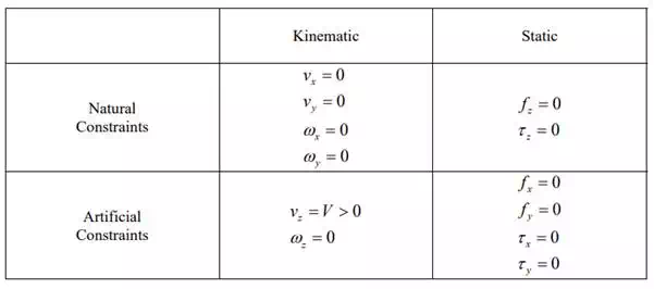
In the statics domain, forces and torques are specified in such a way that the quasi-static condition is satisfied. This means that the peg motion must not be accelerated with any unbalanced force, i.e. non-zero inertial force. Since we have assumed that the process is frictionless, no resistive force acts on the peg in the direction that is not constrained by geometry. Therefore, the linear force in the z direction must be zero: fz = 0 . The rotation about the z axis, too, is not constrained. Therefore, the torque about the z axis must be zero: τ z = 0 . These conditions are dictated by physics, and are called the natural constraints in the statics domain. The remaining directions are geometrically constrained. In these directions, forces and torques can be assigned arbitrarily, and may be controlled with force control mode. The reference inputs to these control loops must be determined so as to meet the task objectives. In this task, it is not required to push the peg against the wall of the hole, nor twist it. Therefore, the reference inputs are set to zero f x = 0, f y = 0, τ x = 0, τ y = 0: . These constitute the artificial constraints in the statics domain.

• Each C-frame axis must have only one control mode, either position or force,

• The process is quasi-static and friction less, and

• The robot motion must conform to geometric constraints.

•

In general, the axes of a C-frame are not necessarily the same as the direction of a separate control mode. Nevertheless, the orthogonality properties hold in general. We prove this next.

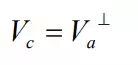
 Let V6 be a six-dimensional vector space, and be an admissible motion space, that is, the entire collection of admissible motions conforming to the geometric constraints involved in a given task. Let Vc be a constraint space that is the orthogonal complement to the admissible motion space:

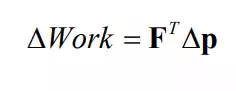
Let  F ∈V be a six-dimensional endpoint force acting on the end-effecter, and be an infinitesimal displacement of the end-effecter. The work done on the end-effecter is given by

Decomposing each vector to the one in the admissible motion space and the one in the constraint space,

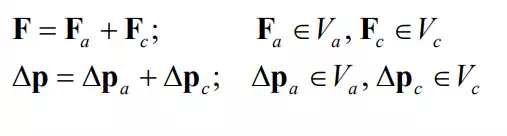
and substituting them to eq.(2) yield

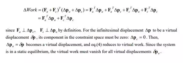
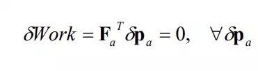
This implies that any force and moment in the admissible motion space must be zero, i.e. the natural static constraints:

The reader will appreciate Mason’s Principle when considering the following exercise problem, in which the partition between admissible motion space and constraint space cannot be described by a simple division of C-frame axes. Rather the admissible motion space lies along an axis where a translational axis and a rotational axis are coupled.