Inertia Matrix
In this section we will extend Lagrange’s equations of motion obtained for the two d.o.f. planar robot to the ones for a general n d.o.f. robot. Central to Lagrangian formulation is the derivation of the total kinetic energy stored in all of the rigid bodies involved in a robotic system. Examining kinetic energy will provide useful physical insights of robot dynamic. Such physical insights based on Lagrangian formulation will supplement the ones we have obtained based on Newton-Euler formulation.
As seen in eq.(3) for the planar robot, the kinetic energy stored in an individual arm link consists of two terms; one is kinetic energy attributed to the translational motion of mass mi and the other is due to rotation about the centroid. For a general three-dimensional rigid body, this can be written as
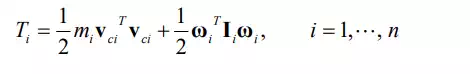
where and Ii are, respectively, the 3x1 angular velocity vector and the 3x3 inertia matrix of the i-th link viewed from the base coordinate frame, i.e. inertial reference. The total kinetic energy stored in the whole robot linkage is then given by
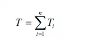
since energy is additive.
The expression for kinetic energy is written in terms of the velocity and angular velocity of each link member, which are not independent variables, as mentioned in the previous section. Let us now rewrite the above equations in terms of an independent and complete set of generalized coordinates, namely joint coordinates q = [q1, .. ,qn] T . For the planar robot example, we used the Jacobian matrix relating the centroid velocity to joint velocities for rewriting the expression. We can use the same method for rewriting the centroidal velocity and angular velocity for three-dimensional multi-body systems.
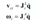
where JL i and JA i are, respectively, the 3 x n Jacobian matrices relating the centroid linear velocity and the angular velocity of the i-th link to joint velocities. Note that the linear and angular velocities of the i-th link are dependent only on the first i joint velocities, and hence the last n-i columns of these Jacobian matrices are zero vectors. Substituting eq.(13) into eqs.(11) and (12) yields
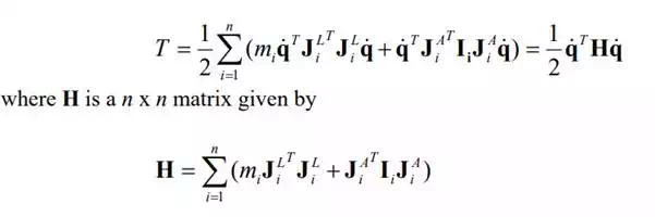
The matrix H incorporates all the mass properties of the whole robot mechanism, as reflected to the joint axes, and is referred to as the Multi-Body Inertia Matrix. Note the difference between the multi-body inertia matrix and the 3 x 3 inertia matrices of the individual links. The former is an aggregate inertia matrix including the latter as components. The multi-body inertia matrix, however, has properties similar to those of individual inertia matrices. As shown in eq. (15), the multi-body inertia matrix is a symmetric matrix, as is the individual inertia matrix defined by eq. (7.1.2). The quadratic form associated with the multi-body inertia matrix represents kinetic energy, so does the individual inertia matrix. Kinetic energy is always strictly positive unless the system is at rest. The multi-body inertia matrix of eq. (15) is positive definite, as are the individual inertia matrices. Note, however, that the multi-body inertia matrix involves Jacobian matrices, which vary with linkage configuration. Therefore, the multi-body inertia matrix is configuration-dependent and represents the instantaneous composite mass properties of the whole linkage at the current linkage configuration. To manifest the configuration-dependent nature of the multi-body inertia matrix, we write it as H(q), a function of joint coordinates q.
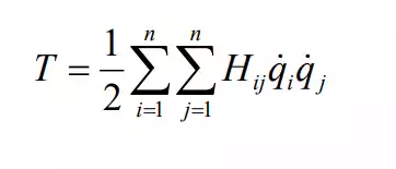
Using the components of the multi-body inertia matrix H={Hij}, we can write the total kinetic energy in scalar quadratic form:
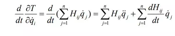
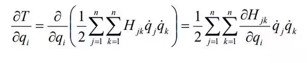
Most of the terms involved in Lagrange’s equations of motion can be obtained directly by differentiating the above kinetic energy. From the first term in eq.(2),
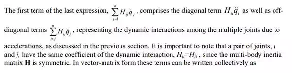
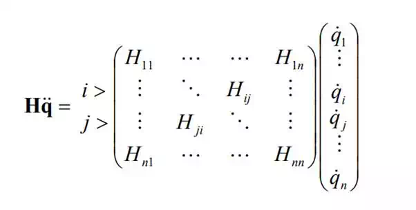
It is clear that the interactive inertial torque caused by the j-th joint acceleration upon the ith joint has the same coefficient as that of caused by joint i upon joint j. This property is called Maxwell’s Reciprocity Relation. Hijqj H jiqi
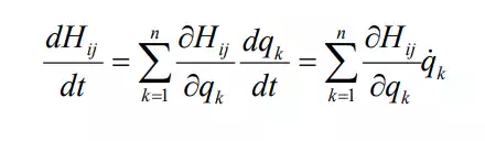
The second term of eq.(17) is non-zero in general, since the multi-body inertia matrix is configuration-dependent, being a function of joint coordinates. Applying the chain rule,
The second term in eq.(2), Lagrange’s equation of motion, also yields the partial derivatives of Hij.
Substituting eq.(19) into the second term of eq.(17) and combining the resultant term with eq.(20), let us write these nonlinear terms as
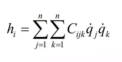
where coefficients Cijk is given by
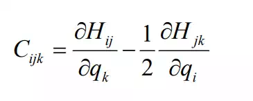
This coefficient Cijk is called Christoffel’s Three-Index Symbol. Note that eq.(21) is nonlinear, having products of joint velocities. Eq.(21) can be divided into the terms proportional to square joint velocities, i.e. j=k, and the ones for j ≠ k : the former represents centrifugal torques and the latter Coriolis torques.
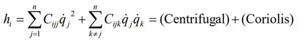
These centrifugal and Coriolis terms are present only when the multi-body inertia matrix is configuration dependent. In other words, the centrifugal and Coriolis torques are interpreted as nonlinear effects due to the configuration-dependent nature of the multi-body inertia matrix in Lagrangian formulation.
Generalized Forces
Forces acting on a system of rigid bodies can be represented as conservative forces and non-conservative forces. The former is given by partial derivatives of potential energy U in Lagrange’s equations of motion. If gravity is the only conservative force, the total potential energy stored in n links is given by
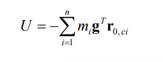
where is the position vector of the centroid Ci that is dependent on joint coordinates. Substituting this potential energy into Lagrange’s equations of motion yields the following gravity torque seen by the i-th joint:
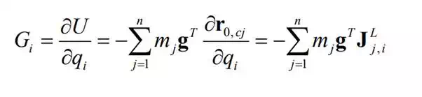
where is the i-th column vector of the 3 x 1 Jacobian matrix relating the linear centroid velocity of the j-th link to joint velocities. L J j,i
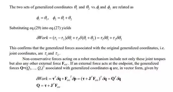
Non-conservative forces acting on the robot mechanism are represented by generalized forces Qi in Lagrangian formulation. Let δWork be virtual work done by all the non-conservative forces acting on the system. Generalized forces Qi associated with generalized coordinates qi, e.g. joint coordinates, are defined by
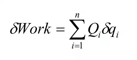
If the virtual work is given by the inner product of joint torques and virtual joint displacements, q nδqn τ δ +"+τ 1 1 , the joint torque itself is the generalized force corresponding to the joint coordinate. However, generalized forces are often different from joint torques. Care must be taken for finding correct generalized forces. Let us work out the following example.
Consider the same 2 d.o.f. planar robot as Example 7.1. Instead of using joint angles θ1 and θ2 as generalized coordinates, let us use the absolute angles, φ1 and φ2 , measured from the positive x-axis. See the figure below. Changing generalized coordinates entails changes to generalized forces. Let us find the generalized forces for the new coordinates.
Absolute joint angles φ1 and φ2 and disjointed links
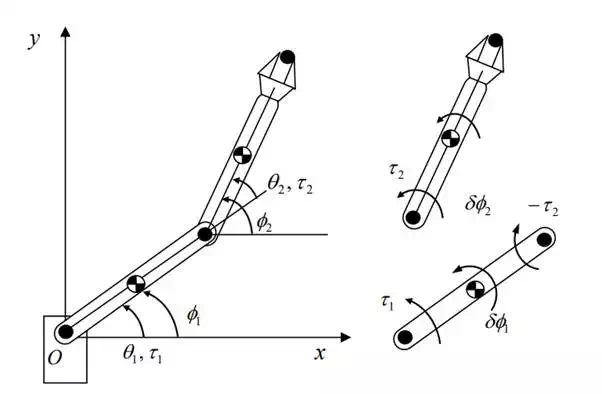
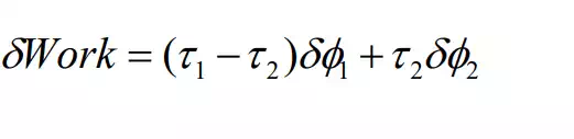
As shown in the figure, joint torque 2 τ acts on the second link, whose virtual displacement is δφ2 , while joint torque 1 τ and the reaction torque 2 −τ act on the first link for virtual displacementδφ1 . Therefore, the virtual work is
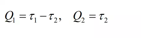
Comparing this equation with eq.(26) where generalized coordinates are 1 1 2 2 φ = q , φ = q , we can conclude that the generalized forces are:
Note that, since generalized coordinates q can uniquely locate the system, the position vector r must be written as a function of q alone.