Inverse Kinematics of Differential Motion
Now that we know the basic properties of the Jacobian, we are ready to formulate the inverse kinematics problem for obtaining the joint velocities that allow the end-effecter to move at a given desired velocity. For the two dof articulated robot, the problem is to find the joint velocities , for the given end-effecter velocity . If the arm configuration is not singular, this can be obtained by taking the inverse of the Jacobian matrix
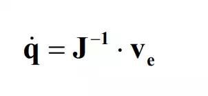
Note that the solution is unique. Unlike the inverse kinematics problem discussed in the previous chapter, the differential kinematics problem has a unique solution as long as the Jacobian is nonsingular.
The above solution determines how the end-effecter velocity ve must be decomposed, or resolved, to individual joint velocities. If the controls of the individual joints regulate the joint velocities so that they can track the resolved joint velocities q , the resultant end-effecter velocity will be the desired ve. This control scheme is called Resolved Motion Rate Control, attributed to Daniel Whitney (1969). Since the elements of the Jacobian matrix are functions of joint displacements, the inverse Jacobian varies depending on the arm configuration. This means that although the desired end-effecter velocity is constant, the joint velocities are not. Coordination is thus needed among the joint velocity control systems in order to generate a desired motion at the end-effecter.
Consider the two dof articulated robot arm again. We want to move the endpoint of the robot at a constant speed along a path staring at point A on the x-axis, (+2, 0), go around the origin through points B (+ε, 0) and C (0, +ε), and reach the final point D (0, +2) on the y-axis. For simplicity, each arm link is of unit length. Obtain the profiles of the individual joint velocities as the end-effecter tracks the path at the constant speed.
trajectory tracking near the singular points
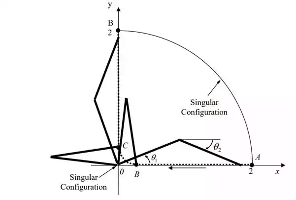
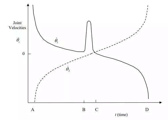
The resolved joint velocities 1 2 computed along the specified trajectory. Note that the joint velocities are extremely large near the initial and final points, and are unbounded at points A and D. These are at the arm’s singular configurations, 2 θ ,θ θ = 0 . As the end-effecter gets close to the origin, the velocity of the first joint becomes very large in order to quickly turn the arm around from point B to C. At these configurations, the second joint is almost –180 degrees, meaning that the arm is near a singularity. This result agrees with the singularity condition using the determinant of the Jacobian:
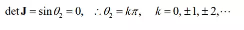
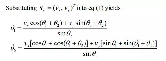
The numerators are divided by 2 sinθ , the determinant of the Jacobian. Therefore, the joint velocities blow up as the arm configuration gets close to the singular configuration.
Joint velocity profiles for tracking the trajectory
Furthermore, the arm’s behavior near the singular points can be analyzed by substituting θ 2 = 0, π into the Jacobian, as obtained. For 1 A1 = A 2 = and 0 θ 2 = , the Jacobian column vectors reduce to the ones in the same direction:
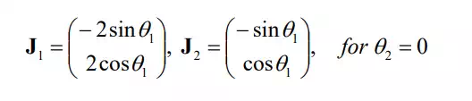
As illustrated (singular configuration A), both joints 1 2 generate the endpoint velocity along the same direction. Note that no endpoint velocity can be generated in the direction perpendicular to the aligned arm links. For θ ,θ θ2 = π ,
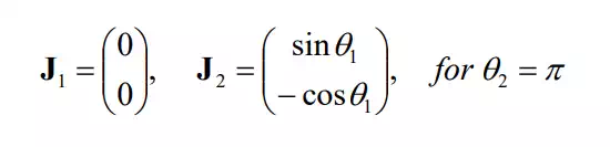
The first joint cannot generate any endpoint velocity, since the arm is fully contracted. See singular configuration B.
At a singular configuration, there is at least one direction in which the robot cannot generate a non-zero velocity at the end-effecter. This agrees with the previous discussion; the Jacobian is degenerate at a singular configuration, and the linear combination of the Jacobian column vectors cannot span the whole space.
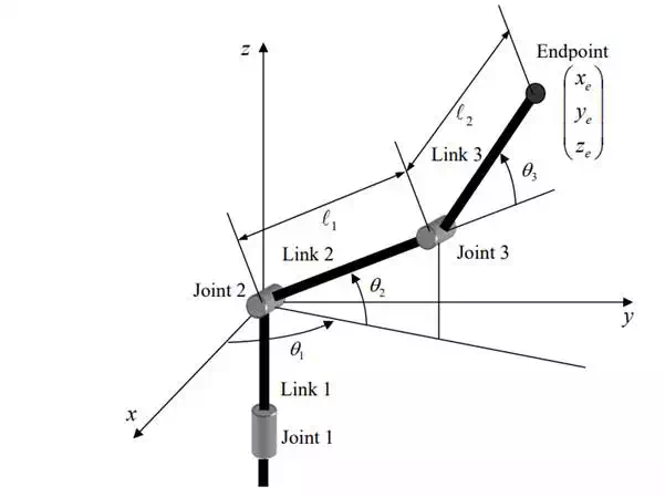
A three-dof spatial robot arm is shown in the figure below. The robot has three revolute joints that allow the endpoint to move in the three-dimensional space. However, this robot mechanism has singular points inside the workspace. Analyze the singularity, following the procedure below
Step 1 Obtain each column vector of the Jacobian matrix by considering the endpoint velocity created by each of the joints while immobilizing the other joints.
Step 2 Construct the Jacobian by concatenating the column vectors and set the determinant of the Jacobian to zero for singularity: detJ = 0 .
Step 3 Find the joint angles that make detJ = 0 .
Step 4 Show the arm posture that is singular. Show where in the workspace it becomes singular. For each singular configuration, also show in which direction the endpoint cannot have a nonzero velocity.
Schematic of a three dof articulated robot
Singularity and Redundancy
We have seen in this chapter that singular configurations exist for many robot mechanisms. Sometimes, such singular configurations exist in the middle of the workspace, seriously degrading mobility and dexterity of the robot. At a singular point, the robot cannot move in certain directions with a non-zero velocity. To overcome this difficulty, several methods can be considered. One is to plan a trajectory of the robot motion such that it will not go into singular configurations. Another method is to include additional degrees of freedom, so that even when some degrees of freedom are lost at a certain configuration, the robot can still maintain the necessary degrees of freedom. Such a robot is referred to as a redundant robot. In this section we will discuss singularity and redundancy and obtain general properties of differential motion for general n degree of freedom robots.
As studied in Section 5.3, a unique solution exists to the differential kinematic equation, (5.3.1), if the arm configuration is non-singular. However, when a planar (spatial) robot arm has more than three (six) degrees of freedom, we can find an infinite number of solutions that provide the same motion at the end-effecter. Consider for instance the human arm, which has seven degrees of freedom excluding the joints at the fingers. When the hand is placed on a desk and fixed in its position and orientation, the elbow position can still vary continuously without moving the hand. This implies that a certain ratio of joint velocities exists that does not cause any velocity at the hand. This specific ratio of joint velocities does not contribute to the resultant endpoint velocity. Even if these joint velocities are superimposed onto other joint velocities, the resultant end-effecter velocity is the same. Consequently, we can find different solutions of the instantaneous kinematic equation for the same end-effecter velocity. In the following, we investigate the fundamental properties of the differential kinematics when additional degrees of freedom are involved.
To formulate a differential kinematic equation for a general n degree-of-freedom robot mechanism, we begin by modifying the definition of the vector dxe representing the end-effecter motion. In eq. (5.1.6), dxe was defined as a two-dimensional vector that represents the infinitesimal translation of an end-effecter. This must be extended to a general m-dimensional vector. For planar motion, m may be 3, and for spatial motion, m may be six. However, the number of variables that we need to specify for performing a task is not necessarily three or six. In arc welding, for example, only five independent variables of torch motion need be controlled. Since the welding torch is usually symmetric about its centerline, we can locate the torch with an arbitrary orientation about the centerline. Thus, five degrees of freedom are sufficient to perform arc welding. In general, we describe the differential end-effecter motion by m independent variables dp that must be specified to perform a given task.
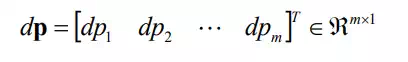
Then the differential kinematic equation for a general n degree-of-freedom robot is given by

where the dimension of the Jacobian J is m by n; . When n is larger than m and J is of full rank, there are (n-m) arbitrary variables in the general solution of eq.(2). The robot is then said to have (n-m) redundant degrees of freedom for the given task. m×n J ∈ℜ
Associated with the above differential equation, the velocity relationship can be written
![]()
where pand qare velocities of the end effecter and the joints, respectively.
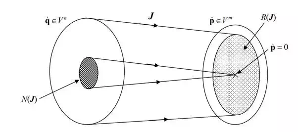
Equation (3) can be regarded as a linear mapping from n-dimensional vector space Vn to m-dimensional space Vm. To characterize the solution to eq.(3), let us interpret the equation using the linear mapping diagram shown in Figure 5.4.1. The subspace R(J) in the figure is the range space of the linear mapping. The range space represents all the possible end-effecter velocities that can be generated by the n joints at the present arm configuration. If the rank of J is of full row rank, the range space covers the entire vector space Vm. Otherwise, there exists at least one direction in which the end-effecter cannot be moved with non-zero velocity. The subspace N(J) of Figure 5.4.1 is the null space of the linear mapping. Any element in this subspace is mapped into the zero vector in Vm. Therefore, any joint velocity vector q that belongs to the null space does not produce any velocity at the end-effecter. Recall the human arm discussed before. The elbow can move without moving the hand. Joint velocities for this motion are involved in the null space, since no end-effecter motion is induced. If the Jacobian is of full rank, the dimension of the null space, dim N(J), is the same as the number of redundant degrees of freedom (n-m). When the Jacobian matrix is degenerate, i.e. not of full rank, the dimension of the range space, dim R(J), decreases, and at the same time the dimension of the null space increases by the same amount. The sum of the two is always equal to n:
dim R(J) + dim N(R) = n
Let q * be a particular solution of eq.(3) and be a vector involved in the null space, then the vector of the form q0 q q* q0 = +k is also a solution of eq.(3), where k is an arbitrary scalar quantity. Namely,
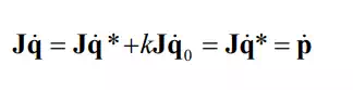
Since the second term can be chosen arbitrarily within the null space, an infinite number of solutions exist for the linear equation, unless the dimension of the null space is 0. The null space accounts for the arbitrariness of the solutions. The general solution to the linear equation involves the same number of arbitrary parameters as the dimension of the null space.
Linear mapping diagram