Inverse Kinematics of Planar Mechanisms

The vector kinematic equation derived in the previous section provides the functional relationship between the joint displacements and the resultant end-effecter position and orientation. By substituting values of joint displacements into the right-hand side of the kinematic equation, one can immediately find the corresponding end-effecter position and orientation. The problem of finding the end-effecter position and orientation for a given set of joint displacements is referred to as the direct kinematics problem. This is simply to evaluate the right-hand side of the kinematic equation for known joint displacements. In this section, we discuss the problem of moving the end-effecter of a manipulator arm to a specified position and orientation. We need to find the joint displacements that lead the end-effecter to the specified position and orientation. This is the inverse of the previous problem and is thus referred to as the inverse kinematics problem. The kinematic equation must be solved for joint displacements, given the end-effecter position and orientation. Once the kinematic equation is solved, the desired end-effecter motion can be achieved by moving each joint to the determined value.

set of joint displacements. On the other hand, the inverse kinematics is more complex in the sense that multiple solutions may exist for the same end-effecter location. Also, solutions may not always exist for a particular range of end-effecter locations and arm structures. Furthermore, since the kinematic equation is comprised of nonlinear simultaneous equations with many trigonometric functions, it is not always possible to derive a closed-form solution, which is the explicit inverse function of the kinematic equation. When the kinematic equation cannot be solved analytically, numerical methods are used in order to derive the desired joint displacements.

Consider the three dof planar arm shown in Figure 4.1.1 again. To solve its inverse kinematics problem, the kinematic structure is redrawn in Figure 4.2.1. The problem is to find three joint angles 1 2 3 θ ,θ ,θ that lead the end effecter to a desired position and orientation, e e e x , y ,φ . We take a two-step approach. First, we find the position of the wrist, point B, from e e e x , y ,φ . Then we find 1 2 θ ,θ from the wrist position. Angle θ3 can be determined immediately from the wrist position.

Skeleton structure of the robot arm

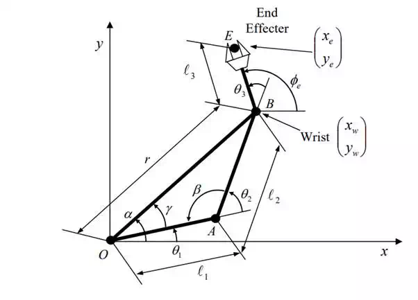
Let w and w be the coordinates of the wrist. As shown in Figure 4.2.1, point B is at distance 3 from the given end-effecter position E. Moving in the opposite direction to the end effecter orientation x y A φe , the wrist coordinates are given by

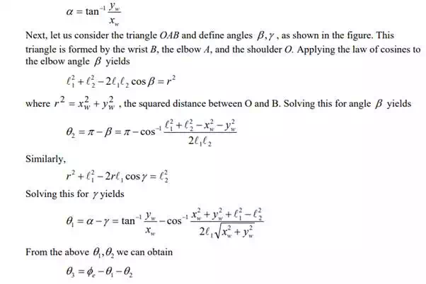
Note that the right hand sides of the above equations are functions of  Xe, Ye ,φe alone. From these wrist coordinates, we can determine the angle α.

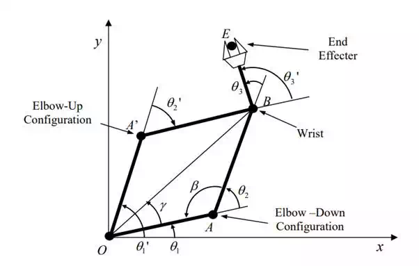
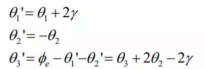
  a set of joint angles that locates the end-effecter at the desired position and orientation. It is interesting to note that there is another way of reaching the same end-effecter position and orientation, i.e. another solution to the inverse kinematics problem. two configurations of the arm leading to the same end-effecter location: the elbow down configuration and the elbow up configuration. The former corresponds to the solution obtained above. The latter, having the elbow position at point A’, is symmetric to the former configuration with respect to line OB, as shown in the figure. Therefore, the two solutions are related as

Inverse kinematics problems often possess multiple solutions, like the above example, since they are nonlinear. Specifying end-effecter position and orientation does not uniquely determine the whole configuration of the system. This implies that vector p, the collective position and orientation of the end-effecter, cannot be used as generalized coordinates.

The existence of multiple solutions, however, provides the robot with an extra degree of flexibility. Consider a robot working in a crowded environment. If multiple configurations exist for the same end-effecter location, the robot can take a configuration having no interference with the environment. Due to physical limitations, however, the solutions to the inverse kinematics problem do not necessarily provide feasible configurations. We must check whether each solution satisfies the constraint of movable range, i.e. stroke limit of each joint.

Multiple solutions to the inverse kinematics problem