Motion Tracking and Potentially Dangerous Situations Recognition in Complex Environment.

Improving safety at level crossing (LC) became an important academic research topic in the transportation field and took increasingly railway undertaking concerns. European countries and European projects try to upgarde level crossing safety which is quite weak today. These projects, like SELCAT “Safer European Level Crossing Appraisal and Technology”, has set up some databases of accidents at European level. United States presents very well equipped level crossing with advanced means for sensing and telecommunication. Selectra Vision Company in Italy has developed a surveillance system for detecting obstacles in the monitored area of a level crossing using a 3D laser scanner. Nevertheless, developing a new LC safety system which allows quantifying the risk within the LC environment and transmitting it to road users, rail managers and even train drivers still is the main focus for technical solutions.

One of the objectives of the proposed work is to perform a video analysis‐based system in order to evaluate the degree of danger of each detected and tracked moving object at level crossing.

The first step of our proposed video surveillance system starts by robustly detecting and separating moving objects crossing the LC. Many approaches are used in the literature to detect objects in real time; examples are Independent Components Analysis, Histogram of Oriented Gradients, Wavelet, Eigen backgrounds, kernel and contour tracking or Kalman and particle filters. However, these techniques require further development to distinguish between detected objects.

That is why our approach consists of detecting all moving pixels based on a background subtraction approach. To obtain separated objects, we propose a model based on clustering the detected pixels, affected by motion, by comparing a specific energy vector associated to each target. Finally, the tracking of each pixel detected within a moving object is achieved by using a Harris corners‐based optical flow propagation technique, followed by a Kalman filtering‐based rectification.

The second step is focused on predicting trajectories of the detected moving objects such as to avoid potentially dangerous level crossing accident scenarios (vehicle stopped at LC for example). Gaussian mixture model (GMM), hidden Markov model (HMM), Hierarchical and Couple Hidden Markov Model are usually used for representing and recognizing objects’ trajectories. However, these methods need a high number of statistical measures to be accurate. Using a real‐time hidden Markov model, the degree of dangerousness related to each object is instantly estimated by analyzing each object’s trajectory considering different sources of danger (position, velocity, acceleration…). All the information obtained from the sources of danger is fused using Dempster‐Shafer technique. Figure 1 illustrates the synopsis of the proposed video surveillance security system.

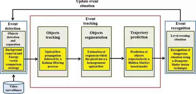
FIGURE 1.

Synoptic of the video surveillance security system installed at Level crossing.

The remaining of the chapter is organized as follows. Section 2 is dealing with object detection and separation. In Section 3, the tracking process is developed. Section 4 describes the proposed method for evaluating and recognizing dangerous situations in a level crossing environment. In Section 5, some evaluation results are provided based on typical accident scenarios played in a real level crossing environment. Finally, in Section 6, some conclusions and short‐term perspectives are provided.

Object detection and separation

In this section, a method has been developed to detect and separate moving objects in the level crossing surveillance zone. This method starts by detecting pixels affected by motion, by using background subtraction technique as a preprocessing phase; each image processed at each step, a subtraction from the background image is carried out. The main aim of this procedure is to extract the moving pixels in the current image (Figure 2b). Furthermore, a subtraction from the previous image is also carried out in order to obtain the moving pixels situated on the edges of the object. (Figure 2c). The procedure continues by determining in the current image the required targets. A target in the image is defined by a set of connected pixels affected by motion. A bounding box is then associated for each group of connected pixels (Figure 3).

FIGURE 2.

Detection of moving pixels. (a) Current image. (b) Detected moving pixels. (c) Moving pixels situated in the contour of the objects.

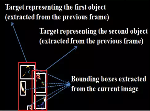
FIGURE 3.

Bounding boxes extraction.

Each created bounding box may belong to an existing target extracted from the previous frame, or representing a new target extracted from the current frame (Figure 3). The intersection between all created bounding boxes in the current frame and those representing the targets extracted from the previous frame is analyzed in order to determine the number and the shape of all moving objects (targets) in the current frame; a bounding box created from the current frame is considered as a new target if and only if it does not intersect any existing bounding box representing a target extracted from the previous frame. On the other case, if a bounding box created from the current frame intersects existing targets, an iterative separation method is applied. During each iteration, a pixel in the current bounding box should be assigned to one of the existing targets.

The pixels clustering process starts by defined two energy vectors. The first energy vector EitargetEtargeti, initialized to zero, is concerned with each existing target number i. This energy is then updated iteratively. The second energy vector EipixelEpixeli is defined for each pixel located at the position (x,y)(x,y) with respect to the target number ii. This energy is expressed as follows:

where EiG, EiI, EiF, EiD are, respectively, the distance, optical flow, intensity and gradient energies.

For each iteration, the pixel (x,y) is assigned to the target that provides the maximum number of closest components between the energy vectors Eipixel and Eitargeti, if the pixel (x,y) is assigned to the target number p. The energy vector Eptarget is then updated as follows:

where NN is the number of pixels in the target number pp, before adding the pixel (x,y). Figure 4 shows the results of the multiobjects separation method.

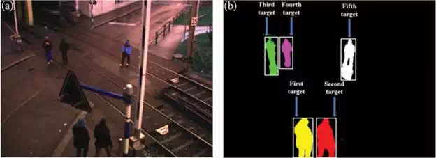
FIGURE 4.

Multiobjects separation result. (a) Original frame with five moving objects. (b) Objects separation result.

Event tracking

OBJECTS TRACKING

Once the targets are extracted from the current frame, the objective is to develop a dense optical flow computation algorithm to track them. We firstly estimate the optical flow of Harris points using an iterative Lucas‐Kanade algorithm. We consider that these particular points have a stable optical flow. The optical flow for every pixel of the detected objects is then estimated by propagating the optical flow of Harris points using a Gaussian distribution. The mean and standard deviation of the distribution are taken as the mean and standard deviation of the Harris points’ optical flow. The results of the optical flow propagation process are then processed by Kalman filtering to correct the optical flow of all the pixels of the detected objects.

The tracking process is tested and evaluated in. Figure 5 shows an example of multiobjects tracking by combining the objects detection and separation method, and the tracking process.

FIGURE 5.

Tracking process: from right to left.

OPTICAL FLOW–BASED OBJECT SEGMENTATION

Given a target, the objective is to partition it into multiple rectangular boxes representing different regions based on optical flow of its pixels. To achieve that, we use a recursive algorithm, which compares neighboring pixels to extract regions in which the pixels have a homogeneous optical flow. Only regions with a significant size are conserved (determined experimentally in dependence of the camera’s view around the level crossing area and the resolution of the camera). Figure 6 presents optical flow–based segmentation results for a moving object tracked in an image sequence. In order to predict the normal (supposed) trajectories, the extracted regions are represented by the gravity centers of the boxes surrounding them. Then, each specific trajectory should be linked to the gravity center of its extracted region.

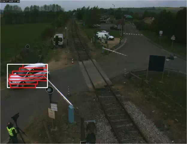
FIGURE 6.

Segmentation of an object using optical flow procedure.

IDEAL TRAJECTORY PREDICTION

Let us consider, thanks to optical flow, an extracted region. When we consider the center of the region, two trajectories could be defined: current ideal trajectory and predicted ideal trajectory. The current ideal trajectory corresponds to the trajectory that the center of the region should follow to avoid potential dangerous situations (Figure 9). The predicted ideal trajectory corresponds to the trajectory that should be followed to come back toward the current ideal trajectory (Figure 7). A statistical approach based on a hidden Markov model (HMM) is proposed to predict the new ideal trajectory: the predicted ideal trajectory of the considered region center at time instant tt (state qtqt: initial state of the HMM) is constructed from the states (qt+1,…, qt+tf)(qt+1,…, qt+tf) generated by the HMM using Forward‐Backward, Viterbi and Baum‐Welch algorithms. We also associate to the considered region center the four following parameters: velocity (Vt+1,…, Vt+tf), acceleration (at+1,…, at+tf), orientation (ot+1,…, ot+tf), position (pt+1,…, pt+tf) and the distance (Dt+1,…, Dt+tf) from the region center to the current ideal trajectory.

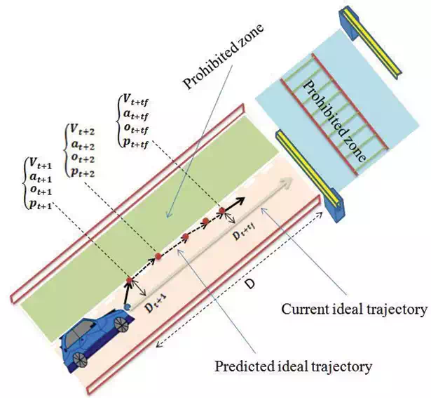
FIGURE 7.

Ideal trajectory prediction by using HMM.

Figure 8 shows the general architecture of the proposed HMM and how the predicted ideal trajectory is performed from the considered region center.

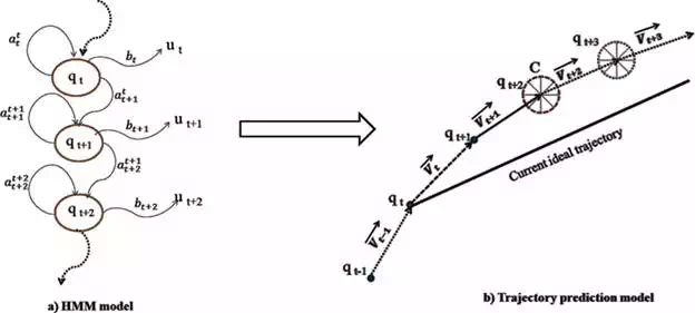
FIGURE 8.

Schematic representation of the HMM for ideal trajectory prediction. (a) HMM model. (b) Trajectory prediction model.

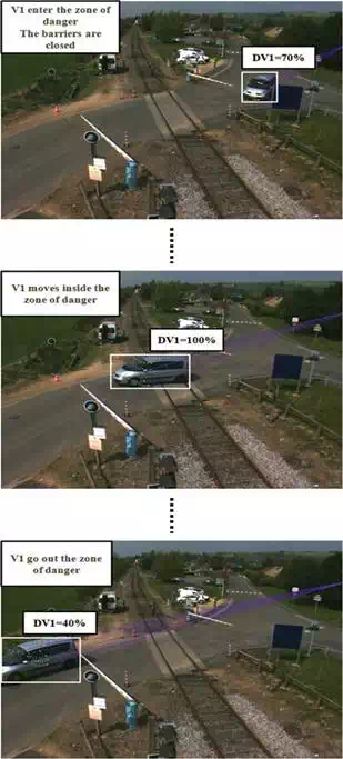
FIGURE 9.

Vehicle zigzagging. DV1 represents the degree of danger associated with the vehicle.

As shown in Figure 8a, the random hidden state variable qtqt corresponds to the position of the considered region center at time t. The random observation variable utut represents simultaneously the acceleration, orientation, velocity and position of the considered region center at time t. att+1at+1t represents the transition probability from state qtqt to state qt+1qt+1, and btbt represents the distribution of the observation at time tt.

As illustrated in Figure 8b, given the velocity vector Vt−→ at time t, calculated from optical flow, the state qt+1 in the HMM is reached from the state qtqt with a probability of 1. Given the acceleration, orientation and velocity at time tt, the velocity Vt+1−→ at time t+1is then predicted. As illustrated in Figure 8b, we next define a circle C. The center of the circle C is the end point of the velocity vector Vt+1−→ and the radius of this circle is the maximum absolute acceleration.

Evaluation of the level of dangerousness (recognition of dangerous situations)

On the basis of the previous steps, we present in this section a method to evaluate and recognize potential dangerous situations when a moving object is detected within the monitored area of a level crossing.

To analyze the predicted ideal trajectory, various sources of dangerousness are considered based on Dempster‐Shafer theory [16]. This theory combines the dangers produced by the different sources in order to obtain a measure of the degree of danger.

For each region center, five sources of danger are considered: acceleration, orientation, velocity, position and distance between the predicted and the current ideal trajectories. A mass assignment is then defined for each source of danger. Let mimi be the belief mass related to the danger source number ii. The belief masses are defined as follows:

The mass assignment m1m1 (position) is computed from the distance between the predicted position pt+tfpt+tfat time instant t+tft+tf and the barrier of the level crossing:

where GdN,σd(x)GdN,σd(x) is a Gaussian distribution of the variable xx. dN=0dN=0 and σdσd are, respectively, its mean and standard deviation. DmaxDmax is the maximum distance that an object can traverse in the image. dtfcdctf is a function given as follows:

where Dp−→=[DpxDpy]T is the distance from the region center to the barrier of the level crossing. Vtfc−→is the velocity of the considered region center at time tftf. The parameter W depends on the position of the region center in the level crossing zone (inside or outside a prohibited LC zone). More the value of dtfcdctf is greater than zero more the belief mass m1m1 will increase (degree of dangerousness increments).

The mass assignment m2m2 (velocity) is computed from the difference between the predicted velocity Vtfcat time instant tf and a prefixed nominal velocity VN.

where Vtfc is the velocity of the considered region center at time tftf. VN represents the maximal velocity that a target can reach in the image. GVn,σv(x) is a Gaussian distribution, with a mean equal to VN and a standard deviation equal to σv.

The mass assignment m3m3 (orientation) is computed by comparing the angle of the predicted velocity Vt at time instant t and the angle of the current ideal trajectory.

where otfc is the velocity orientation of the considered region center at time tf. ON is the orientation of the current ideal trajectory. GoN,σo(x) is a Gaussian distribution, with a mean equal to ON and a standard deviation equal to σo.

The mass assignment m4 (acceleration) is computed from the difference between the predicted accelerations at and at+tf  at time instants t and t+tf respectively.

where atfc is the acceleration of the considered region center at time tftf. aN represents the maximal acceleration that a target can reach in the image. GaN,σa(x) is a Gaussian distribution, with a mean equal to aN and a standard deviation equal to σa.

Finally, the mass assignment m5 (distance) is computed from the distance between the predicted position ptf time instant tf  and the current ideal trajectory:

where Dtf is the the distance between the predicted position ptf of the considered region center at time tftf and the current ideal trajectory. GDN,σD(x) is a Gaussian distribution, with a mean equal to DN=0 and a standard deviation equal to σD.

Once the degrees of dangerousness are computed for the five sources, Dempster‐Shafer combination is used to determine the degree of danger related to the considered region center:

To determine the degree of danger of the target, we take simply the maximum value among the degrees of danger of all regions composing the target.

Video surveillance experimental results

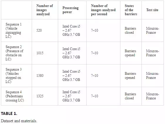
To validate our work, we apply the proposed dangerous situation method on four typical accidental scenarios. These scenarios, registered at a level crossing in the north of France (Mouzon), correspond to real situations occurred in LC accidents (dangerous situations: vehicle zigzagging between the closed half barriers, presence of obstacle in the level crossing and pedestrian crossing level crossing area). Each analyzed scenario includes a sequence with more than 500 frames. Table 1 presents the datasets and materials used in the analysis of our method.

EXPERIMENTAL METHODOLOGY

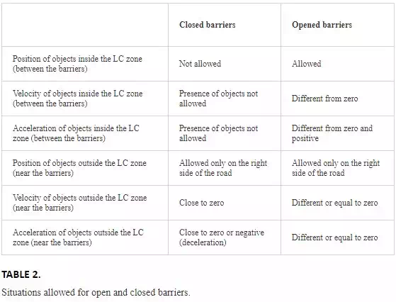
In the framework of this chapter, we determine a pure quantitative degree of dangerousness from different scenarios identified at level crossing (see Eq. (18)). This system is able to detect potentially dangerous situations occurring at the LC both in the two cases (states of the barriers): barriers opened or barriers closed.

In the case of closed barriers, when train approaching, we provide a level of dangerousness (see Eq. (18)), between 0 and 100%, which could be transmitted all the time to the drivers approaching the level crossing (LC). We could also send additional security advices when the level is greater than a threshold (for instance 75%). In any situation, the presence of any kind of moving objects between the barriers is not allowed. So, the velocity of cars or moving objects should decrease to zero when approaching the LC.

In the case of opened barriers, the surveillance system is working as well. Vehicles or moving objects could traverse the level crossing zone but they couldn’t stop on the LC. In case of detection of dangerous situations, we can send information like: barriers open with a pedestrian, a vehicle or an object stopped on the rails.

Table 2 shows different situations that are taken into account by the system to measure the level of dangerousness. In both cases, it all depends on the way of the rail transport operator wants to monitor the LC. For the moment, the final system was not integrated in the daily management of a level crossing. So, when the system will be integrated in a rail network, we could imagine that the measure of the level of dangerousness will be validated qualitatively by the rail safety experts.

SCENARIOS OF ACCIDENT ANALYZED BY THE SYSTEM

Vehicle zigzagging between two closed barriers of LC (Figure 9): In this scenario, a vehicle is approaching the LC, while the barriers are closed. The vehicle crosses the LC, zigzagging between the closed barriers (Figure 9). The purple lines in Figure 9 represent the current ideal trajectory of the center of each extracted region from the object. The white points in the figure represent the instantly predicted displacement of the center of the extracted regions. As shown in Figure 9, if a detected vehicle is approaching the LC and using an abnormal trajectory, the degree of danger is going to increase gradually to reach 70%. Then, when the vehicle enters the LC, this degree continues to grow until reaching 100%. The level of danger begins to decrease when the vehicle is moving away from the LC (Degree of danger DV1 = 40%).

Vehicle stopped (Figure 10): In this scenario, a vehicle crosses the level crossing while the barriers are open (Figure 10). Suddenly, the vehicle stops inside the dangerous zone and becomes a fixed obstacle. After a while, the vehicle moves and leaves the LC. Concerning danger evaluation, the degree of dangerousness related to the detected vehicle increases when it moves toward the level crossing. It reaches 46% during the crossing of the zone of danger. When the vehicle stops in the zone of danger, the stationary is detected and the degree of dangerousness takes a value of 100%. When the vehicle begins to leave the LC, the level of danger decreases progressively.

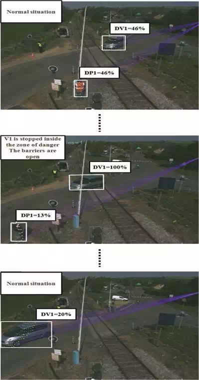
FIGURE 10.

The presence of obstacle (vehicle) in the level crossing. DV1 represents the degree of danger associated with the vehicle.

Queuing across the rail level crossing (Figure 11): In this scenario, a first vehicle stops just after the dangerous zone. Sometime later, two other vehicles find themselves blocked behind the first vehicle, which is motionless. This situation leads to a queue of cars inside the LC (Figure 11). When the two vehicles detected inside the LC are stopped inside the zone of danger, their degree of dangerousness increases progressively and reach their maximum (100%). When the two vehicles restart moving, the degree of dangerousness drops to 46% and decreases gradually, as the vehicles leave away the level crossing.

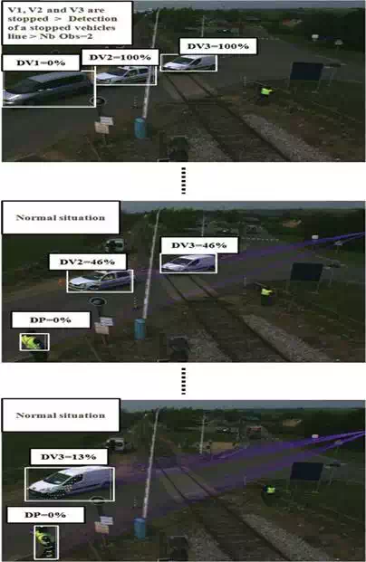
FIGURE 11.

The presence of stopped vehicles line on the LC. DVi represents the degree of danger associated with the vehicle number i. DP represents the degree of danger associated with a pedestrian outside the LC zone.

Pedestrians’ scenario (Figure 12): In this scenario, three pedestrians (P1, P2 and P3) are walking around the level crossing zone as the barriers are closed. Pedestrian P1 is moving toward the zone of danger (Degree of danger DP1 = 26%), while pedestrian P2 is crossing is crossing the level crossing area (DP2 = 100%), and Pedestrian P3 is stopped on the middle part of the level crossing near from the rails (DP3 = 100%). After a moment, pedestrian P1 arrives near pedestrian P2, and they are stopped on the rails of the LC, taking into account that the stationary inside the level crossing is always detected by the system. So, the degree of dangerousness related to the pedestrian P1 increases progressively from DP1 = 26% and reaches their maximum DP1 = 100% on the rails. At the end of the scenario, pedestrian P2 is leaving the level crossing zone (Degree of danger DP2 decreases to 11%), when pedestrian P1 is moving toward the stopped pedestrian P3. A vehicle passing near from the LC is also detected in this scenario (DV = 13%).

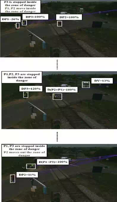
FIGURE 12.

Three pedestrians walking around the level crossing area.

As a conclusion of these tests, the measure of the prediction system that calculates the level of dangerousness for each moving or stopped object around the LC is able to detect different kind of dangerous scenarios in the case of closed or opened barriers (vehicle zigzagging, stopped vehicles, pedestrians around the LC). Then, this system proves his effectiveness as a measure of the level of dangerousness but it also requires to be validated qualitatively after installing this system definitely on a rail transport.

Conclusion

Detection of moving objects is an important and basic task for video surveillance systems, for which you can define the initial position of the moving objects in a surveillance scene. However, the detection and separation of the moving objects process become difficult when the objects are close to each other in the scene. In our approach, we propose a method to completely separate the corresponding pixels of each defined target. One of the other objectives of this project is to develop a video surveillance system that will be able to detect and recognize potential dangerous situation around level crossings. Different typical LC accident scenarios (e.g., presence of obstacles, zigzagging between the barriers, stopped cars line) acquired in real conditions are experimentally evaluated by applying the proposed dangerous situation recognition system.