Audio-Visual Speaker Tracking

Speaker tracking aims at localizing the moving speakers in a scene by analysing the data sequences captured by sensors or arrays of sensors. It gained relevance in the past decades due to its widespread applications such as automatic camera steering in video conferencing, individual speaker discriminating in multi‐speaker environments, acoustic beamforming, audio‐visual speech recognition, video indexing and retrieval, human‐computer interaction, and surveillance and monitoring in security applications. There are numerous challenges, which make speaker tracking a difficult task including, but not limited to, the estimation of the variable number of speakers and their states, and dealing with various conditions such as occlusions, limited view of cameras, illumination change and room reverberations.

Using multi‐modal information is one way to address these challenges since more comprehensive observations for the state of the speakers can be collected in multi‐modal tracking as compared to the single‐modal case, and the collection of the multi‐modal information can be achieved by sensors such as audio, video, thermal vision, laser‐range finders and radio‐frequency identification (RFID). Among these sensors, audio and video sensors are commonly used in speaker tracking compared to others, because of their easier installation, cheaper cost and more data‐processing tools.

Earlier methods in speaker tracking employ either visual‐only or audio‐only data, and each modality offers some advantages but is also limited by some weaknesses. Tracking with only video offers robust and accurate performance when the camera field of view covers the speakers. However, it degrades when the occlusion between speakers happens, when the speakers go out of the camera field of view, or any changes on illumination or target appearance have occurred. Although audio tracking is not restricted by these limitations, it has a tendency to non‐negligible‐tracking errors because of intermittency of audio data. In addition, audio data may be corrupted by background noise and room reverberations. Nevertheless, the combination of audio and video data may improve the tracking performance when one of the modalities is missing or neither provides accurate measurements, as audio and visual modalities are often complementary to each other which can be exploited to further enhance their respective strengths and mitigate their weaknesses in tracking.

Previous techniques were focused on tracking a single person in a static and controlled environment. However, theoretical and algorithmic advances together with the increasing capability in computer processing have led to the emergence of more sophisticated techniques for tracking multiple speakers in dynamic and less controlled (or natural) environments. In addition, the type of sensors used to collect the measurements is advanced from single‐ to multi‐modal.

In the literature, there are many approaches for speaker tracking using multi‐modal information, which can be categorized into two methods as one is deterministic and data‐driven while the other is stochastic and model‐driven. Deterministic approaches are considered as an optimization problem by minimizing a cost function, which needs to be defined appropriately. A representative method in this category is the mean‐shift method, which defines the cost function in terms of colour similarity measured by Bhattacharyya distance. The stochastic and model‐driven approaches use a state‐space approach based on the Bayesian framework as it is suitable for processing of multi‐modal information. Representative methods are the Kalman filter (KF), extended KF (EKF) and particle filter (PF). The PF approach is more robust for non‐linear and non‐Gaussian models as compared with the KF and EKF approaches since it easily approaches the Bayesian optimal estimate with a sufficiently large number of particles.

One challenge in the implementation of the PF to tracking problem is to choose an optimal number of particles. An insufficient number may introduce a particle impoverishment, while a larger number (than required) will lead to extra computational cost. Therefore, choosing the optimal number of particles is one of the issues that affect the performance of the tracker. To address this issue and to find the optimal number of particles for the PF to use, adaptive particle filtering (A‐PF) approaches have been proposed in Refs. Fox proposed KLD sampling, which aims to bind the error introduced by the sample‐based representations of the PF using the Kullback‐Leibler divergence between maximum likelihood estimates (MLEs) of the states and the underlying distribution to optimize the number of particles. The KLD‐sampling criterion is improved in Ref. for the estimation of the number of particles, leading to an approach for adaptive propagation of the samples. Subsequent work introduces the innovation error to estimate the number of particles by employing a twofold metric. The particles are removed by the first metric in case their distance to a neighbouring particle is smaller than a predefined threshold. The second metric is used to set the threshold on the innovation error in order to control the birth of the particles. These two thresholds need to be set before the algorithm is run. A new approach is proposed in Refs., which estimates noise variance besides the number of particles in an adaptive manner. Different from other existing adaptive approaches, adaptive noise variance is employed in this method for the estimation of the optimal number of particles based on tracking error and the area occupied by the particles in the image.

One assumption in the traditional PF used in multi‐speaker tracking is that the number of speakers is known and invariant during the tracking. In practice, the presence of the speakers may change in a random manner, resulting in time‐varying number of speakers. To deal with the unknown and variable number of speakers, the theory of random finite sets (RFSs) has been introduced, which allows multi‐speaker filtering by propagation of the multi‐speaker posterior. However, the computational complexity of RFS grows exponentially as the number of speakers increases since the complexity order of the RFS is O(MΞ) where M is the number of measurements and Ξ is the number of speakers. The PHD filtering approach is proposed to overcome this problem, as the first‐order approximation of the RFS whose complexity scales linearly with the number of speakers since the complexity order of the PHD is O(MΞ). This framework has been found to be promising for multi‐speaker tracking. However, the PHD recursion involves multiple integrals that need to have closed‐form solutions for implementation. So far, two analytic solutions have been proposed: Gaussian mixture PHD (GM‐PHD) filter and sequential Monte Carlo PHD (SMC‐PHD) filter. Applications of GM‐PHD filter are limited by linear Gaussian systems, which lead us to consider SMC‐PHD filter to handle non‐linear/non‐Gaussian problems in audio‐visual tracking.

Apart from the stochastic methodologies mentioned above, the mean-shift is a deterministic and data‐driven method, which focuses on target localization using representation of the target. The mean-shift easily convergences to peak of the function with a high speed and a small computational load. Moreover, as a non‐parametric method, the solution of the mean shift is independent from the features used to represent the targets. On the other hand, the performance of the mean-shift is degraded by occlusion or clutter as it searches the densest (most similar) region starting from the initial position in the region of interest. In this sense, the mean‐shift trackers may fail easily in tracking small‐ and fast‐moving targets as the region of interest may not cover the targets, which results in a track being lost after a complete occlusion. Also, it is formulated for single‐target tracking, so it cannot handle a variable number of targets. Therefore, several methods have been proposed by integrating both deterministic and stochastic approaches to benefit their respective strengths which will be discussed in Section 4.

Tracking modalities

VISUAL CUES

Visual tracking is a challenging task in real‐life scenarios, as the performance of a tracker is affected by the illumination conditions, occlusion by background objects and fast and complicated movements of the target. To address these problems, several visual features, that is, colour, texture, contour and motion, are employed in existing tracking systems.

Using colour feature is a very intuitive approach and commonly applied in target tracking as the information provided by colour helps to distinguish between targets and other objects. Several approaches can be found in the literature which employs colour information to track the target. In Ref., a colour mixture model based on a Gaussian distribution is used for tracking and segmentation, while in Ref., an adaptive mixture model is developed. Target detection and tracking can be easily maintained using colour information if the colour of the target is distinct from those of the background or other objects.

Another approach for tracking is contour‐based where shape matching or contour‐evolution techniques are used to track the target contour. Active models like snakes, geodesic‐active contours, B‐splines or meshes can be employed to represent the contours. Occlusion of the target by other objects is the common problem in tracking. This problem can be addressed by detecting and tracking the contour of the upper body rather than tracking the contour of the whole bodies, which leads to the detection of a new person as the upper bodies are often distinguishable from back and front view for different people.

Texture is another cue defined as a measure for surface intensity variation. Properties like smoothness and regularity can be quantified by the texture. The texture feature is used with Gabor wavelet in Ref.. The Gabor filters can be employed as orientation and scale‐tunable edge and line detectors, and the statistics of these micro‐features are mostly used to characterize the underlying texture information in a given region. For improved detection and recognition, local patterns of image have gained attention recently. Local patterns are used in several application areas such as image classification and face detection since they offer promising results. In Ref., the local binary patterns (LBPs) method is used to create a type of texture descriptor based on a grey‐scale‐invariant texture measure. Such a measure is tolerant to illumination changes.

Another cue used in tracking, particularly in indoor environments, is motion which is an explicit cue of human presence. One way to extract this cue is to apply foreground detection algorithms. A simple method for foreground detection is to compute the difference of two consecutive frames which gives the moving part of the image. Although it has been used in multi‐modal‐tracking systems, it fails when the person remains stationary since the person is considered part of background after some time.

The scale‐invariant feature transform (SIFT) proposed in Ref. has found wide use in tracking applications. SIFT uses local features to transform the image data into scale‐invariant coordinates. Distinctive invariant features are extracted from images to provide matching between several views of an object. The SIFT feature is invariant to scaling, translation, clutter, rotation, occlusion and lighting which makes it robust to changes in three‐dimensional (3D) viewpoint and illumination, and the presence of noise. Even a single feature has high matching rate in a large database because the SIFT features are generally distinctive. On the other hand, non‐rigid targets in noisy environments degrade the SIFT matching rate and recognition performance.

So far, several visual cues were introduced, and among them colour cues have been used more commonly in tracking applications due to their easy implementation and low complexity. Colour information can be used in the calculation of the histogram of possible targets at the initialization step as reference images which can be used in detection and tracking of the target. There are two common colour histogram models, RGB or HSV in the literature and HSV is more preferable since it is observed to be more robust to illumination variation.

AUDIO CUES

There are a variety of audio information that could be used in audio tracking such as sound source localization (SSL), time‐delay estimation (TDE) and the direction of arrival (DOA) angle.

The audio source localization methods can be divided into three categories, namely steered beamforming, super‐resolution spectral estimation and time‐delay estimation. Beamformer‐based source localization offers comparatively low resolution and needs a search over a highly non‐linear surface. Also, it is computationally expensive which may be limited in real‐time applications. Super‐resolution spectral estimation methods are not well suited for locating a moving speaker since it is under the assumption that the speaker location is fixed for a number of frames. However, the location of a moving speaker may change considerably over time. In addition, these methods are not robust to modelling errors caused by room reverberation and mostly have high computational cost. The time‐delay of arrival (TDOA)‐based location estimators use the relative time delay between the wave‐front arrivals at microphone positions in order to estimate the location of the speaker. As compared with the other two methods, the TDOA‐based approach has advantages in the following two aspects. The first one is its computational efficiency and the second one its direct connection to the speaker location.

The problem of DOA estimation is similar to that of the TDOA estimation. To estimate the DOA, the TDOA needs to be determined between the sensor elements of the microphone array. Estimation of source locations mainly depends on the quality of the DOA measurements. In the literature, several DOA estimation techniques such as the MUSIC algorithm and the coherent signal subspace (CSS) have been proposed. The main differences between them are the way of dealing with reverberation, background noise and movement of the sources. The following three factors influence the quality of the DOA estimation. The spectral content of the speech segment is considered as the first one which is used for derivation of the DOAs. The reverberation level of the room is the second one which causes outlier in the measurements because of the reflections from the objects and walls. The positions of the microphone array to the speakers and the number of simultaneous sources in the field are considered the third factor.

Audio‐visual speaker tracking

Speaker tracking is a fundamental part of multimedia applications which plays a critical role to determine the speaker trajectories and analyse the behaviour of speakers. Speaker tracking can be accomplished with the use of audio‐only, visual‐only or audio‐visual information.

Audio‐only information based approaches for speaker tracking have been presented in. An audio‐based fusion scheme was proposed in Ref. to detect multiple speakers where the locations from multiple microphone arrays are estimated and fused to determine the state of the same speaker. Separate KFs are employed for all the individual microphone arrays for the location estimation. To deal with motion of the speaker and measurement uncertainty, the probabilistic data association technique is used with an interacting model.

One issue in Ref. is that it cannot deal with the tracking problem for a time‐varying number of speakers. Ma et al. proposed an approach based on random finite set to track an unknown and time‐varying number of speakers. The RFS theory and SMC implementation are used to develop the Bayesian RFS filter, which tracks the time‐varying number of speakers and their states. The random finite set theory can deal with a time‐varying number of speakers; however, the maximum number of speakers that can be handled is limited as its computational complexity increases exponentially with the number of speakers. In that sense, a cardinalized PHD (CPHD) filter is proposed in Ref., which is the first‐order approximation of the RFS, to reduce the computational cost caused by the number of speakers. The positions of the speakers are estimated using TDOA measurements from microphone pairs by asynchronous sensor fusion with the CPHD filter.

A time‐frequency method and the PHD filter are used in Ref. to localize and track simultaneous speakers. The location of multiple speakers is estimated based on the time‐frequency method, which uses an array of three microphones, then the PHD filter is employed to the localization results as post‐processing to handle miss‐detection and clutters.

Speaker tracking with multi‐modal information has also gained attention, and many approaches have been proposed in the past decade using audio‐visual information , providing the complementary characteristics of each modality. The differences among these existing works arise from the overall objective such as tracking either single or multiple speakers and the specific detection/tracking framework.

Audio‐visual measurements are fused by graphical models in Ref. to track a moving speaker in a cluttered and noisy environment. Audio and video observations are used jointly by computing their mutual dependencies. The model parameters are learnt using the expectation‐maximization algorithm from a sequence of audio‐visual data.

A hierarchical Kalman filter structure was proposed in Refs. to track people in a three‐dimensional space using multiple microphones and cameras. Two independent local Kalman filters are employed for audio and video streams, and then the outputs of these two local filters are combined under one global Kalman filter.

Unlike particle filters to estimate the predictions from audio‐ and video‐based measurements and audio‐visual information fusion is performed at the feature level. In other words, the independent particle coordinates from the features of both modalities are fused for speaker tracking. These works have focused on the single‐speaker case which cannot directly address the tracking problem for multiple speakers.

Two multi‐modal systems are introduced in Ref. for the tracking of multiple persons. A joint probabilistic data association filter is employed to detect speech and determine active speaker positions. Two systems are performed for visual features where a particle filter is applied first using foreground, colour, upper body detection and person region cues from multiple camera images and the latter is a blob tracker using only a wide‐angle overhead view. Then, acoustic and visual tracks are integrated using a finite state machine. Unlike, a particle filtering framework is proposed in Ref. which incorporates the audio and visual detections into the particle filtering framework using an observation model. It has the capability to track multiple people jointly with their speaking activity based on a mixed‐state dynamic graphical model defined on a multi‐person state space. Another particle filter based multi‐modal fusion approach is proposed in Ref. where a single speaker can be identified in the presence of multiple visual observations. Gaussian mixtures model was adopted to fuse multiple observations and modalities. Compared to, particle filtering framework is not used in Ref.; instead, hidden Markov model based iterating decoding scheme is used to fuse audio and visual cues for localization and tracking of persons.

In Refs., the Bayesian framework is used to handle the tracking problem for a varying number of speakers. The particle filter is used in Ref., and observation likelihoods based on both audio and video measurements are formulated to use in the estimation of the weights of the particles, and then the number of people is calculated using the weights of these particles. The RFS theory based on multi‐Bernoulli approximations is employed in Ref. to integrate audio and visual cues with sequential Monte Carlo implementation. The nature of the random finite set formulation allows their framework to deal with the tracking problem for a varying number of targets. Sequential Monte Carlo implementation (or particle filter) of PHD filter is used in Ref. where audio and visual modalities are fused in the steps of particle filter rather than using any data fusion algorithms. Their work substantially differs from existing works in AV multi‐speaker tracking with respect to the capabilities for dealing with multiple speakers, simultaneous speakers, and unknown and time‐varying number of speakers.

Tracking algorithms

In this section, a brief review of tracking algorithms is presented which covers the following topics: Bayesian statistical methods, visual and audio‐visual algorithms and non-linear filtering approaches.

Recall that in Section 1, tracking methods are either stochastic and model‐driven or deterministic and data‐driven.

The stochastic approaches are based on the Bayesian framework which uses a state‐space approach. Representative methods in this category are the Kalman filter (KF), extended Kalman filter (EKF) and particle filter (PF). The PF approach is more robust as compared to the KF and EKF approaches as it can approach the Bayesian optimal estimate with a sufficiently large number of particles. It has been widely applied to speaker tracking problems. The PF is used to fuse object shapes and audio information in Refs. In Ref., independent audio and video observation models are fused for simultaneous tracking and detection of multiple speakers. However, one challenge in PF is to choose an appropriate number of particles. While an insufficient number may lead to particle impoverishment (i.e. loss of diversity among the particles), a larger number (than required) will induce additional computational cost. Therefore, the performance of the tracker depends on the number of particles that are estimated as an optimal value.

The PHD filter is another stochastic method based on the finite‐set statistics (FISST) theory, which propagates the first‐order moment of a dynamic point process. The PHD filter is used in many application areas after its proposal and some applications with speaker tracking are reported in Refs. It has an advantage over other Bayesian approaches such as Kalman and PF filters, in that the number of targets does not need to be known in advance since it is estimated in each iteration. The issue in the PHD filter is that it is prone to estimation error in the number of speakers in the case of low signal‐to‐noise ratio. The reason is that the PHD filter restricts the propagation of multi‐target posterior to the first‐order distribution moment, resulting in loss of information for higher order cardinality. To address this issue, the cardinality distribution is also propagated with PHD distribution in the cardinalized PHD (CPHD) filter which improves the estimation of the target number and state of the speakers. However, additional distribution for cardinality requires extra computational load, which makes the CPHD computationally more expensive than the PHD filter. Moreover, the spawning of new targets is not modelled explicitly in the CPHD filter.

As a deterministic and data‐driven method, the mean-shift uses representation of the target for localization, which is based on minimizing an appropriate cost function. In that sense, a similarity function is defined in Ref. to reduce the state estimation problem to a search in the region of interest. To obtain fast localization, a gradient optimization method is performed. The mean-shift works under the assumption that the representation of the target is sufficiently distinct from the background which may not be always true. Although the mean-shift is an efficient and robust approach, in occlusion and rapid motion scenarios, it may fail when the target is out of the region of interest, in other words, the search area.

Many approaches have been proposed in the literature to address these problems in mean‐shift tracking, which can be categorized into two groups. One group improves the mean‐shift tracking by, for example, introducing adaptive estimation of the search area, iteration number and bin number. In the other group, the mean‐shift algorithm is combined with other methods such as particle filter. The stochastic and deterministic approaches are integrated under the same framework in many studies. Particle filtering (stochastic) is integrated with a variation approach (deterministic) in Ref. where the ‘switching search’ algorithm is run for all the particles. In this algorithm, the momentum of the particles is compared with a pre‐determined threshold value, and if it is smaller than the threshold, the deterministic search is run; otherwise, the particles are propagated in terms of a stochastic motion model.

The particle filtering and mean-shift are combined in Ref. under the name of mean-shift embedded particle filter (MSEPF). It is inspired by Sullivan and Rittscher, but the mean shift is used as a variational method. It is aimed to integrate the advantages of the particle filtering and mean‐shift method. The MSEPF has a capability to track the target with a small number of particles as the mean‐shift search concentrates on the particles around local modes (maxima) of the observation. To deal with the possible changes in illuminations, a skin colour model is used and updated for every frame. As an observation model, colour and motion cues are employed. To use a multi‐cue observation model, the mean‐shift analysis is modified and applied to all the particles. Resampling (selective resampling) is, then, applied when the effective sample size is too small. The mean‐shift and particle filtering methods are used independently in Ref. The estimated positions of the target obtained by these two methods are compared using the Bhattacharyya distance at every iteration and the best value is chosen as the estimated position of the target to avoid the algorithm from being trapped to a local maximum, and thus finding the true maximum beyond the local one.

A hybrid particle with a mean‐shift tracker is proposed in Ref. which works in a similar manner to that in Ref. Alternatively, uses the original application of the mean-shift and performs the mean‐shift process on all the particles to reach the local maxima. Moreover, an adaptive motion model is used to deal with manoeuvring targets, which have a high speed of movement. The kernel particle filter is proposed in Ref. where small perturbations are added to the states of the particles after the mean‐shift iteration to prevent the gradient ascent from being stopped too early in the density. Kernel radius is calculated adaptively every iteration and this method is applied to multiple target tracking using multiple hypotheses which are then evaluated and assigned to possible targets. An adaptive mean‐shift tracking with auxiliary particles is proposed in Ref. As long as the conditions are met, such as the target remaining in the region of interest, and there are no serious distractions, the mean-shift is used as the main tracker. When sudden motions or distractions are detected by the motion estimator, auxiliary particles are introduced to support the mean‐shift tracker. As the mean shift may diverge from the target and converge on the background, background/foreground feature selection is applied to minimize the tracking error. Even though this study is inspired by Sullivan and Rittscher, where the main tracker is a particle filter, in Ref., the main tracker is the mean-shift. In addition, the switched trackers are used to handle sudden movements, occlusion and distractions. Moreover, to maintain tracking even when the target appearance is affected by illumination or view point, the target model is updated online.

In the literature, several frameworks have been proposed to combine the mean-shift and particle filters. However, it is still required to have an explicitly designed framework for a variable number of targets. Both the mean-shift and particle filter were derived for tracking only a single target. To address this issue, the PHD filter is found as a promising solution as it is originally designed for multi‐target tracking. However, the PHD filter does not have closed‐form solutions as the recursion of the PHD filter includes multi‐dimensional integrals. To derive analytical solution of the PHD filter, the particle filter or sequential Monte Carlo (SMC) implementation is introduced which leads to SMC‐PHD filtering. In Ref., the mean-shift is integrated with standard SMC‐PHD filtering, aiming at improving computational efficiency and estimation accuracy of the tracker for a variable number of targets.

Besides the tracking methods explained so far, speaker tracking with multi‐modal usage introduces a problem which is known as data association. Each measurement coming from multi‐modality needs to be associated with an appropriate target. Data association methods are divided into two classes. Unique neighbour is the first data association, and a representative method in this class is multiple hypothesis tracking (MHT). Here, each existing track is associated with one of the measurements. All‐neighbours data association belongs to the second class which uses all the measurements for updating the entire track estimate, for example, the joint probabilistic data association (JPDA). In MHT, the association between a target state and the measurements is maintained by multiple hypotheses. However, the required number of hypotheses increases exponentially over time. In JPDA, separate Gaussian distributions for each target are used to approximate the posterior target distribution which results in an extra computational cost. Data association algorithms in target‐tracking applications with Bayesian methods and the PHD filter can be found in. However, it is found that classical data association algorithms are computationally expensive which lead to the fusion of multi‐modal measurements inside the proposed framework. As in Refs., audio and visual modalities are fused in the steps of the visual particle filter.

Among the methods explained above, the PF, RFS, PHD filter and mean-shift are the main methods discussed throughout this chapter and the main concepts of the methods are presented below.

PARTICLE FILTERING

The PF became widely used tools in tracking after being proposed by Isard et al. due to its ability to handle non‐linear and non‐Gaussian problems. The main idea of the PF is to represent a posterior density by a set of random particles with associated weights, and then compute estimates based on these samples and weights. The principle of the particle filter is illustrated in Figure 1. Ten particles are initialized with equal weights in the first step. In the second step, the particles are weighted based on given measurements, and as a result, some particles require small weights while others require larger weights represented by the size of the particles. The state distribution is represented by these weighted particles. Then, a resampling step is performed which selects the particles with large weights to generate a set of new particles with equal weights in the third step. In step four, these new particles are distributed again to predict the next state. This loop continues from steps two through four until all the observations are exhausted.

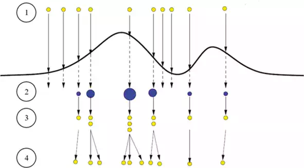
FIGURE 1.

Steps of the particle filter. The first step is particle initialization with equal weights. The particles are weighted in the second step. After a resampling step is performed in the third step, the particles are distributed to predict the next state in the fourth step. This figure is adapted from Ref.

Although there are various extensions of the PF in the literature, the basic concept is the same and based on the idea of representing the posterior distribution by a set of particles.

RANDOM FINITE SET AND PHD FILTERING

The generic PF is designed for single‐target tracking. Multi‐target tracking is more complicated than single‐target tracking as it is necessary to jointly estimate the number of targets and the state of the targets. One multi‐target tracking scenario is illustrated in Figure 2a, where five targets exist in state space (bottom plane) given at the previous time with eight measurements in observation space (upper plane). In this scenario, the number of measurements is larger than the number of targets due to clutter or noise. When the targets are passed to the current time, the number of targets becomes three and two targets no longer exist.

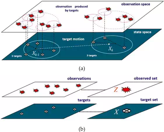
FIGURE 2.

An illustration of the RFS theory in a multi‐target tracking application. One possible multi‐target tracking scenario is given in (a), and (b) represents the RFS approach to multi‐target tracking. The figures are adapted from Ref.

In that sense, the variable number of targets and noisy measurements need to be handled for reliable tracking in multi‐target case. The RFS approach is an elegant solution to address this issue. The basic idea behind the RFS approach is to treat the collection of targets as a set‐valued state called the multi‐target state and the collection of measurements as a set‐valued observation, called multi‐observation. So, the problem of estimating multiple targets in the presence of clutter and uncertainty is handled by modelling these set‐valued entities as random finite sets. The point here is to generalize the tracking problem from single target to multiple targets.

Figure 2b illustrates the RFS approach where all the targets are collected in one target set and all the measurements are considered as one measurement set. The RFS propagates the full multi‐target posterior for multi‐target filtering. The state model of the RFS incorporates individual target dynamics which are target birth, target spawn and target death. In addition, the observation model of the RFS incorporates the measurement likelihood as target detection uncertainty (miss‐detection) and clutter (false alarm). These incorporations are implemented by assigning hypotheses, and all possible associations between hypotheses and measurement/targets need to be repeated at every time step, resulting in increased computational cost in the case of a high number of targets and measurements.

To alleviate the computational cost, the PHD filter is introduced which is a computationally cheaper alternative to the RFS. The PHD filter is the first‐order approximation of the RFS and propagates only the first‐order moments instead of the full multi‐target posterior. The PHD filter function is denoted as the intensity v(x)v(x) whose integral on any region of the state space gives the expected number of targets. The peaks of the PHD function point the highest local concentration of the expected number of targets, which can be used to provide estimates of individual target. The PHD filter is illustrated in Figure 3 by a simple example which corresponds to Eq. (1)

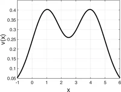
FIGURE 3.

A simple example for the PHD filter. This figure is adapted from Ref..

Figure 3 is plotted for Eq. (1) with σ=1, a=1 and b=4. The peaks of v(x)) is near the target locations x=1 and x=4.

The integral of v(x) computes the actual number of targets Ξ:

MEAN‐SHIFT TRACKING

Different from stochastic approaches such as the PF, RFS and PHD filter, the mean-shift is a deterministic method. The mean-shift can be defined as a simple iterative procedure that shifts each data point to the average of data points in its neighbourhood.

Common application areas are clustering, mode seeking, image segmentation and tracking. Simple implementation of the mean‐shift method is illustrated in Figure 4 where the purpose is to find the densest region of the distributed balls. The first step is to select an initial point with the region of interest as shown in Figure 4a where the circle indicates the region of interest centred on the initial point. In Figure 4b, the centre of the mass is calculated using the balls inside the region of interest. To get the distance and direction for shifting the initial point, the mean‐shift vector is calculated in Figure 4c. The initial point is shifted to a new point together with the region of interest in Figure 4d. The centre of the mass is calculated again using the balls inside the region of interest which leads to new mass point in Figure 4e. The mean‐shift vector is calculated to obtain the direction and distance for shifting and the region of interest is shifted to a new point as illustrated in Figures 4f and g, respectively. This iteration continues until the mean‐shift method reaches the densest point in Figure 4h.

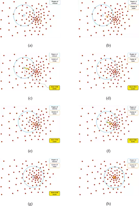
FIGURE 4.

Simple descriptions of the mean‐shift process. These figures are adapted from Ref.

Relevant datasets

In order to perform a quantitative evaluation of the audio‐visual tracker, both audio and video sequences are required. In that sense, several datasets are presented in the literature that combine multiple audio and video sources for tracking.

The augmented multi‐party interaction (AMI) corpus includes 100 h of meetings, which were recorded in English using three different rooms. Natural conversations are included in some of the meetings, and many others, in particular those using a scenario in which the participants play different roles in a design team, are also reasonably natural. The number of speakers in the natural conversations varies from three to five. In one artificial meeting, four speakers are involved, taking four pre‐arranged roles (as industrial designer, interface designer, marketing and project manager). Other artificial meetings also appear in the AMI corpus, such as a film club scenario. Generally, the speakers are mostly static or with small movements. In addition, calibration information is not available which is required for 3D tracking as it is needed to project the coordinates from the two‐dimensional (2D) image into 3D space.

CLEAR (CLassification of Events, Activities and Relationships) is the next dataset created for people identification, activities, human‐human interaction and relevant scenarios. Recordings are captured with multiple users in realistic meeting rooms equipped with a multitude of audio‐visual sensors. The rooms have five calibrated cameras, and four of them are mounted to the corners of the room while the last panoramic camera is mounted to the ceiling of the room. All cameras are synchronized with the audio streams collected by the linear microphone array placed on the walls. In most scenarios, the speakers are generally still and seated around the table. They speak one by one.

Another dataset is SPEVI (Surveillance performance evaluation initiative) created for single‐ and multi‐modal people detection and tracking. Sequences are captured by a video camera and two linear microphone arrays. The SPEVI dataset has three sequences. The sequences motinas_Room160 and motinas_Room105 are captured in rooms with reverberation. The sequence motinas_Chamber is captured in a reduced reverberation room. In this dataset, audio signals were recorded with linear microphone arrays and the calibration information is not available.

One of the most challenging datasets that can be used for the evaluation of audio‐visual tracking algorithm is AV16.3 corpus which is developed by the IDIAP research institute. The corpus AV16.3 involves various scenarios where subjects are moving and speaking at the same time whilst being recorded by three calibrated video cameras and two circular eight‐element microphone arrays.

Recordings in the AV16.3 involve challenging scenarios such as object initialization, partial and total occlusion, overlapped speech, illumination change, close and far locations, variable number of objects, and small and large angular separations. Circular microphone arrays were used to record the audio signals at 16 kHz and video sequences were captured at 25 Hz. The recordings of audio and video were performed independently from each other. Each video frame is a colour image of 288 × 360 pixels and some sequences are annotated to get the ground truth (GT) speaker position which allows one to measure the accuracy of each tracker and to compare the performance of the algorithms. In addition, it provides calibration information of the cameras and challenging scenarios like occlusions and moving speakers.

The most recently released dataset is ‘S3A speaker tracking with Kinect2’ which uses a Kinect for Windows V2.0 for recording the visual data and dummy head for recording the audio data. It contains four sequences in a studio where people are talking and walking slowly around a dummy head which is located at the centre of the room. Different from other cameras, Kinect sensor provides in‐depth information besides the colour which helps to extract the 3D position of the speaker without using additional view of the scene. In addition, annotated data are provided which can be used as ground truth data to estimate the performance of the tracker.

Performance metrics

Several metrics have been proposed to evaluate the performance of tracking methods in the literature. In this section, four metrics are introduced.

The first one is the mean absolute error (MAE), which is computed as the Euclidean distance in pixels between the estimated and the ground truth positions, and then divided by the number of frames. This metric offers simplicity and explicit output for the performance comparison.

The multiple object tracking (MOT) metric is the next metric which was proposed in Ref. It is defined with MOT precision (MOTP) and MOT accuracy (MOTA) quantities. The precision is measured with the MOTP using a pre‐defined threshold value

where dikdki is the distance between the ith object and its corresponding hypothesis and ckck is the number of matches between the objects and hypotheses for time frame kk.

Tracking errors are measured with the MOTA which covers the false positives, false negatives and mismatches. If the error is greater than the threshold value, it is assumed that the false positive and false negative count if the speaker is not tracked with the accuracy measured by the threshold. Mismatches are the case where the speaker identity is switched

where mkmk, fpk, mmk and gkgk define the number of misses (false negatives), false positives, mismatches and objects present, respectively, for the time frame kk.

The next metric is the trajectory‐based measures (TBMs) proposed in Refs., where the performance is measured based on trajectory. It categorizes the trajectories as mostly tracked (MT), mostly lost (ML) and partially tracked (PT). MT is defined as if the tracker follows at least 80% of its ground truth (GT) trajectory. If the tracker follows less than 20% of its GT, it is called ML. If the followed trajectory is between 20 and 80% of the GT trajectory, it is called PT. Also, track fragmentation (Frag) is defined as the total number of times that GT is interrupted. Identity switches (IDs) are computed by calculating change in GT identity.

OSPA‐T (Optimal Subpattern Assignment for Tracks) is the last performance metric designed for the evaluation of multi‐speaker tracking systems. It is an improved version of the OSPA metric by extending it for tracking management evaluation. To transfer the cardinality error into the state error, a penalty value is used in the OSPA. So its performance evaluation includes both source number estimation and speaker position estimation:

 defined as the cut‐off value in order to weight the penalties for cardinality and localization errors. Additionally, the metric order is defined by aa which determines the sensitivity to outliers. The OSPA‐T metric differs from other metrics since it considers not only the position estimation of the speaker but also the estimation of the number of speakers in the evaluation of the tracking results. As OSPA‐T measures the error based on these two terms, state (position estimation) and cardinality (number of speaker estimation), it causes ambiguities about how much error is contributed from each term to the final error. In addition to the x1x1 and x2 variables of the state vector, the scale variable, s, may be considered in the evaluation. However, this will cause more ambiguities in the contributions of the terms to the final error and deteriorate the reliability of the metric.

As a summary, four metrics are introduced which evaluate the methods from their own perspectives. To see how well the tracker follows its trajectory, the TBM can be used to measure its performance. If the tracking error needs to be estimated, the MAE or the more advanced option MOT can be used to see how accurately the tracker follows the target. If an unknown and variable number of targets need to be tracked, then the OSPA‐T metric is more suitable than the others as it considers both position estimation and the estimated number of targets in the performance evaluation.

Experimental results and analysis

In this chapter, six trackers are included to cover the recent paradigms. The trackers are restricted to the ones either for which access to the source code has been permitted or tracker performance has been reported on commonly used datasets.

To deal with the tracking problem for unknown and time‐varying number of speakers, Kılıç et al. propose to use particle PHD (SMC‐PHD) filter. DOA information is employed as an audio cue and it is integrated with video data under SMC‐PHD filter framework. Audio data are used to determine when to propagate and re‐allocate surviving, spawned and born particles based on their types. The particles are concentrated around the DOA line, which is drawn from the centre of the microphone array to the estimated speaker position by audio information.

As a baseline algorithm, the visual SMC‐PHD (V‐SMC‐PHD) filter, which uses colour information as a visual cue, is compared with the audio‐visual SMC‐PHD (AV‐SMC‐PHD) to see the advantage of using multi‐modal information in challenging tracking scenarios like occlusion. Sequence 24 from AV16.3 dataset is run for V‐SMC‐PHD and AV‐SMC‐PHD, and tracking results are given in Figure 5.

FIGURE 5.

AV16.3, sequence 24 camera #1: occlusions with two speakers. Performance of the V‐SMC‐PHD filter is shown in the first row. The second row is given for the AV‐SMC‐PHD filter.

The first row shows the results of V‐SMC‐PHD filter which fails to track after occlusion. Also, it shows poor performance before the occlusion in terms of the detection of the speakers. It is reported in Ref. that the AV‐SMC‐PHD filter tracks the speakers more accurately and shows better performance than the V‐SMC‐PHD filter in terms of accuracy and ability for re‐detection of the speakers after lost.

The same experiments are repeated for three‐speaker case using Sequence 45 camera #3 from the AV16.3 dataset and the results are given in Figure 6. It is reported in Ref. that AV‐SMC‐PHD filter has better capability in detecting and following all the speakers even after the occlusions.

FIGURE 6.

AV16.3, sequence 45 camera #3: occlusions with three speakers. The tracking results of the V‐SMC‐PHD and the AV‐SMC‐PHD filters are shown in the first and second rows, respectively.

To improve the estimation accuracy of the AV‐SMC‐PHD filter, integrates the mean‐shift method in order to shift the particles to a local maximum of the distribution function which drives particles closer the speaker position. The generic mean‐shift algorithm is modified for multiple‐speaker case and applied after the audio contribution to the particles, and this algorithm is named as AVMS‐SMC‐PHD filter.

Even though the integration of the mean-shift improves the estimation accuracy, applying the mean‐shift process to all the particles introduces extra computational cost. To address this problem, proposes a sparse sampling scheme which chooses sparse particles and runs the mean‐shift method only on those particles rather than all the particles which results in a significant reduction in computational cost. This method is named as sparse‐AVMS‐SMC‐PHD filter. Another tracking algorithm is given in Ref., which uses the merits of dictionary learning for multi‐speaker tracking. It is tested using some sequences (seq24, seq25 and seq30) of the AV16.3 dataset.

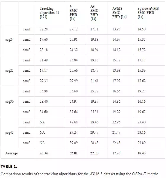
The results of these five trackers on sequences of AV16.3 are given in Table 1 and the OSPA‐T metric is used for comparison. The tracker in Ref. outperforms the V‐SMC‐PHD; however, the AVMS‐SMC‐PHD shows better performance than the others.

These tracking results are compared with those of which uses the PHD filter for tracking and reports the results only for seq24 cam1 and cam2 in terms of Wasserstein distance. Table 2 shows the results of six trackers.

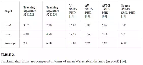
Among six trackers, the AVMS‐SMC‐PHD outperforms the other trackers in terms of the average accuracy.

The trackers of are also tested in different datasets. One sequence from each AMI and CLEAR dataset is used to test the trackers. Figure 7 shows the results of V‐SMC‐PHD and AV‐SMC‐PHD for a sequence of the AMI dataset. In this dataset, the speakers talk one by one. Hence, one DOA line is drawn per time instance. Since the speakers remain still, the visual trackers do not fail to track the speakers.

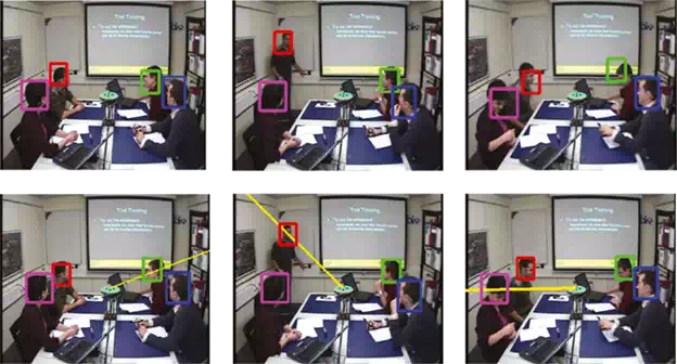
FIGURE 7.

AMI dataset, sequence IS1001a. The first and second rows show the results of the V‐SMC‐PHD and the AV‐SMC‐PHD filter, respectively.

Other sequence is UKA_20060726 from the CLEAR dataset where the speakers talk one by one and mostly sit around the table. The performance of visual and audio‐visual trackers is given in Figure 8.

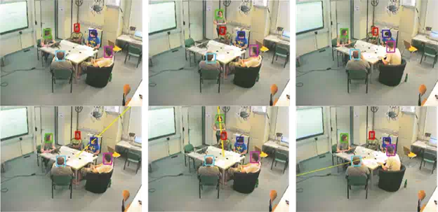
FIGURE 8.

CLEAR dataset, sequence UKA_20060726. The first and second rows show the results of the V‐SMC‐PHD and the AV‐SMC‐PHD filters, respectively.

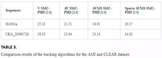
The average error of the trackers for sequences IS1001a and UKA_20060726 is given in Table 3 in terms of the OSPA‐T metric. It is reported in Ref. that there is no significant difference on the performance of the visual and audio‐visual trackers since the speakers talk one by one. The audio‐visual tracker runs as a visual tracker for the silent speakers, while it is more effective for the talking speakers because of the additional information coming from audio modality.

Chapter summary

In this chapter, a review of multi‐speaker tracking has been provided on modalities, existing tracking techniques, datasets and performance metrics that have been developed over the past few decades.

After a broad survey of the tracking methods, a technical background of the methods such as particle filtering, random finite set, PHD filter and mean-shift, which are commonly used as baseline methods in the literature, is introduced with their basic mathematical, statistical concepts and definitions, which are required for understanding the mathematics and techniques behind the proposed tracking algorithms.

In order to perform a quantitative evaluation of the proposed algorithms, both audio and video sequences are required. Publicly available datasets such as AV16.3, CLEAR, AMI, SPEVI and S3A were introduced with the fundamental differences including physical setup, scenarios and challenges.

Moreover, performance metrics were analysed in order to see which aspects are considered more in the evaluation and impacts of these perspectives on the evaluation results.