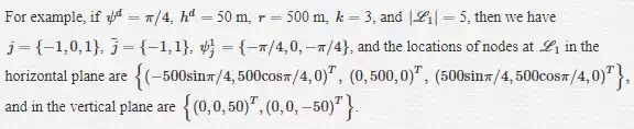
Path Planning in the Local-Level Frame for Small Unmanned Aircraft Systems

The rapid growth of the unmanned aircraft systems (UASs) industry motivates the increasing demand to integrate UAS into the U.S. national airspace system (NAS). Most of the efforts have focused on integrating medium or larger UAS into the controlled airspace. However, small UASs weighing less than 55 pounds are particularly attractive, and their use is likely to grow more quickly in civil and commercial operations because of their versatility and relatively low initial cost and operating expense.

Currently, UASs face limitations on their access to the NAS because they do not have the ability to sense-and-avoid collisions with other air traffic . Therefore, the Federal Aviation Administration (FAA) has mandated that UASs were capable of an equivalent level of safety to the see-and-avoid (SAA) required for manned aircraft . This sense-and-avoid (SAA) mandate is similar to a pilot’s ability to visually scan the surrounding airspace for possible intruding aircraft and take action to avoid a potential collision.

Typically, a complete functional sense-and-avoid system is comprised of sensors and associated trackers, collision detection, and collision avoidance algorithms. In this chapter, our main focus is on collision avoidance and path planning. Collision avoidance is an essential part of path planning that involves the computation of a collision-free path from a start point to a goal point while optimizing an objective function or performance metric. A robust collision avoidance logic considers the kinematic constraints of the host vehicle, the dynamics of the intruder’s motion, and the uncertainty in the states estimate of the intruder. The subject of path planning is very broad, and in particular collision, avoidance has been the focus of a significant body of research especially in the field of robotics and autonomous systems. Kuchar and Yang provided a detailed survey of conflict detection and resolution approaches. Albaker and Rahim conducted a thorough survey of collision avoidance methods for UAS. The most common collision avoidance methods are geometric-based guidance methods, potential field methods, sampling-based methods, cell decomposition techniques, and graph-search algorithms.

Geometric approaches to collision avoidance are straightforward and intuitive. They lend themselves to fast analytical solutions based on the kinematics of the aircraft and the geometry of the encounter scenario. The approach utilizes the geometric relationship between the encountering aircraft along with intuitive reasoning. Generally, geometric approach assumes a straight-line projection to determine whether the intruder will penetrate a virtual zone surrounding an ownship. Then, the collision avoidance can be achieved by changing the velocity vector, assuming a constant velocity model. Typically, geometric approaches do not account for uncertainty in intruder flight plans and noisy sensor information.

The potential field method is another widely used approach for collision avoidance in robotics. A typical potential field works by exerting virtual forces on the aircraft, usually an attractive force from the goal and repelling forces from obstacles or nearby air traffic. Generally, the approach is very simple to describe and easy to implement. However, the potential field method has some fundamental issues. One of these issues is that it is a greedy strategy that is subject to local minima. However, heuristic developments to escape the local minima are also proposed in the literature. Another problem is that typical potential field approaches do not account for obstacle dynamics or uncertainly in observation or control. In the context of airborne path planning and collision avoidance, Bortoff presents a method for modeling a UAS path using a series of point masses connected by springs and dampers. This algorithm generates a stealthy path through a set of enemy radar sites of known locations. McLain and Beard present a trajectory planning strategy suitable for coordinated timing for multiple UAS. The paths to the target are modeled using a physical analogy of a chain. Similarly, Argyle et al. present a path planner based on a simulated chain of unit masses placed in a force field. This planner tries to find paths that go through maxima of an underlying bounded differentiable reward function.

Sampling-based methods like probability road maps (PRM) and rapidly exploring random trees (RRTs) have shown considerable success for path planning and obstacle avoidance, especially for ground robots. They often require significant computation time for replanning paths, making them unsuitable for reactive avoidance. However, recent extensions to the basic RRT algorithm, such as chance-constrained RRT^* and close-loop RRT, show promising results for uncertain environments and nontrivial dynamics. Cell decomposition is another widely used path planning approach that partitions the free area of the configuration space into cells, which are then connected to generate a graph. Generally, cell decomposition techniques are considered to be global path planners that require a priori knowledge of the environment. A feasible path is found from the start node to the goal node by searching the connectivity graph using search algorithms like A^* or Dijkstra’s algorithm.

The proposed approach in this work will consider encounter scenarios such as the one depicted in Figure 1, where the ownship encounters one or more intruders. The primary focus of this work is to develop a collision avoidance framework for unmanned aircraft. The design, however, will be specifically tailored for small UAS. We assume that there exists a sensor(s) and tacking system that provide states estimate of the intruder’s track.

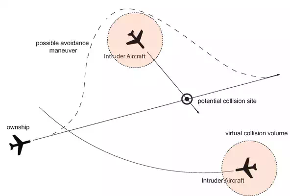
FIGURE 1.

The geometry of an encounter scenario.

Local-level path planning

A collision event occurs when two aircraft or more come within the minimum allowed distance between each other. The current manned aviation regulations do not provide an explicit value for the minimum allowed distance. However, it is generally understood that the minimum allowed or safe distance is required to be at least 500 ft. to 0.5 nautical miles (nmi). For example, the near midair collision (NMAC) is defined as the proximity of less than 500 ft. between two or more aircraft. Similarly and since the potential UAS and intruder aircraft cover a wide range of vehicle sizes, designs, airframes, weights, etc., the choice of a virtual fixed volume boundary around the aircraft is a substitute for the actual dimensions of the intruder.

As shown in Figure 2, the choice for this volume is a hockey-puck of radius dsds and height hshs that commonly includes a horizontal distance of 500 ft. and a vertical range of 200 ft. Accordingly, a collision event is defined as an incident that occurs when two aircraft pass less than 500 ft. horizontally and 100 ft. vertically.

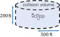
FIGURE 2.

A typical collision volume or protection zone is a virtual fixed volume boundary around the aircraft.

In this work, we develop the path planning logic using a body-centered relative coordinate system. In this body-centered coordinate system, the ownship is fixed at the center of the coordinate system, and the intruder is located at a relative position prpr and moves with a relative velocity vrvr with respect to the ownship.

We call this body-centered coordinate frame the local-level frame because the environment is mapped to the unrolled, unpitched local coordinates, where the ownship is stationary at the center. As depicted in Figure 3, the origin of the local-level reference is the current position of the ownship. In this configuration, the xx-axis points out the nose of the unpitched airframe, the yy-axis points points out the right wing of the unrolled airframe, and the zz-axis points down forming a right-handed coordinate system. In the following discussion, we assume that the collision volume is centered at the current location of the intruder. A collision occurs when the origin of the local-level frame penetrates the collision volume around the intruder.

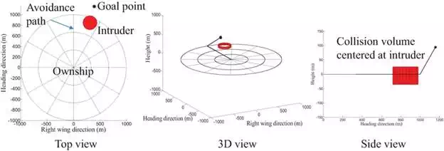
FIGURE 3.

Local-level reference frame.

The detection region is divided into concentric circles that represent maneuvers points at increasing range from the ownship as shown in Figure 4, where the radius of the outmost circle can be thought of as the sensor detection range. Let the region in the space covered by the sensor be called the workspace. Then, this workspace is discretized using a cylindrical grid in which the ownship is commanded to move along the edges of the grid. The result is a directed weighted graph, where the edges represent potential maneuvers, and the associated weights represent the maneuver cost and collision risk. The graph can be described by the tuple G(N,E,C)GNEC, where NN is a finite nonempty set of nodes, and EEis a collection of ordered pairs of distinct nodes from NN such that each pair of nodes in EE is called a directed edge or link, and CC is the cost associated with traversing each edge.

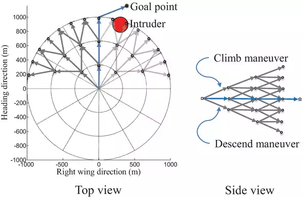
FIGURE 4.

Discretized local-level reference workspace. The three concentric circles represent three maneuvers points.

The path is then constructed from a sequence of nonrepeated nodes n1,n2,⋯,nN such that each consecutive pair ni,ni+1 is an edges in GG. Let the detection range drdr be the radius of the outermost circle, and rr be the radius of the innermost circle so that dr=mrdr=mr. As shown in Figure 6, let Ll l=1,2,⋯,m be the llth level curve of the concentric circles. Assume that the level curves are equally partitioned by a number of points or nodes such that any node on the llth level curve, Ll connects to a predefined number of nodes kk in the next level, that is, in the forward direction along the heading axis as depicted in Figure 4. The nodes on the graph can be thought of as predicted locations of the ownship over a look-ahead time window. Additionally, we assume that only nodes along the forward direction of the heading axis, that is, x=0 connect to nodes in the vertical plane. This assumption allows to command the aircraft to climb or descend by connecting to nodes in the vertical plane as shown in Figure 4. Let the first level curve of the innermost circle be discretized into |L1|=k+2 nodes including nodes in the vertical plane. Then, using the notation |A|A to denote the cardinality of the discrete set AA, the number of nodes in the llth level curve is given by

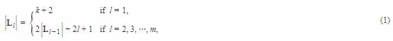
where the total number of nodes is |N|=∑ml=1|Ll|. For example, assuming that the start node is located at the origin of the reference map and given that k = 3, that is, allowing the ownship to fly straight or maneuver right or left. The total number of nodes in the graph including the start and destination node is given by

Figure 5 shows an example of a discretized local-level map. In this example, k= 3 and m= 3, and the total number of nodes in the graph |N| is 39.

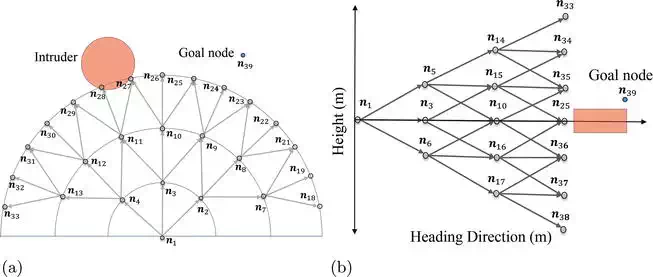
FIGURE 5.

Example of discretized local-level map. (a) Top view: location and index of nodes and (b) side view: location and index of nodes.

Assuming that the ownship travels between the nodes with constant velocity and climb rate, the location of the iith node at the llth level curve, and ni,lni,l in the horizontal plane of the graph is given by

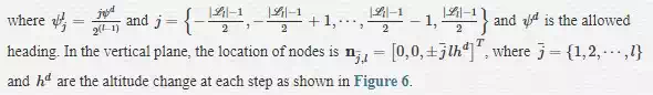
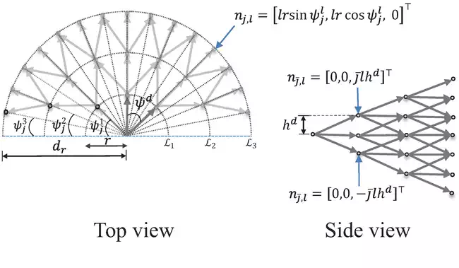
FIGURE 6.

Nodes location in the local-level reference frame.

The main priority of the ownship where it is under distress is to maneuver to avoid predicted collisions. This is an important note to consider when assigning a cost of each edge in the resulting graph. The cost associated with traveling along an edge is a function of the edge length and the collision risk. The cost associated with the length of the edge ei,i+1ei,i+1 that connects between the consecutive pair nodes (ni,ni+1) is simply the Euclidean distance between the nodes nini and ni+1 expressed as

The collision cost for traveling along an edge is determined if at any future time instant, the future position of the ownship along that edge is inside the collision volume of the predicted location of an intruder. An exact collision cost computation would involve the integration of collision risk along each edge over the look-ahead time window τ∈[t,t+mT]

A simpler approach involves calculating the collision risk cost at several locations along each edge, taking into account the projected locations of the intruder over the time horizon ττ. Assuming a constant velocity model, a linear extrapolation of the current position and velocity of the detected intruders are computed at evenly spaced time instants over the look-ahead time window. The look-ahead time interval is then divided into several discrete time instants. At each discrete time instant, all candidate locations of the ownship along each edge are checked to determine whether it is or will be colliding with the propagated locations of the intruders. For the simulation results presented in this chapter, the collision risk cost is calculated at three points along each edge in GG. If vo is the speed of the ownship, then the distance along an edge is given by voT, where T=r/vo. The three points are computed as

Where Ts=T/3. Let the relative horizontal and vertical position of the intruder with respect to the ownship at the current time tt be pr(t) and prz(t), respectively. Define the collision volume as

The predicted locations of each detected intruder over time horizon T at three discrete time samples Ts are

where ℓ={1,2,3}ℓ=123. In Eq. (12), the ∞∞ or the maximum allowable cost is assigned to any edge that leads to a collision, basically eliminating that edge and the path passing through it. The total collision risk associated with the iith edge is given by

where MM is the number of detected intruders.

A visual illustration of the collision risk computation is shown in Figure 7. The propagated collision volume of a detected intruder and the candidate locations of the ownship over the first-time interval [t+Ts,t+3Ts] both in the horizontal and vertical plane is depicted in Figure 7a and b. Clearly, there is no intersection between these candidate points the ownship may occupy and the propagated locations of the collision volume over the same interval. Then, according to Eq. (13), the cost assigned to these edges is zero. Next, all candidate locations of the ownship along each edge over the second time interval [t+4Ts,t+6Ts] are investigated. As shown in Figure 7c, edges e2,7 e2,8 and e2,9 intersect with the predicted intruder location at time t+4TS and t+5TS, respectively. Similarly, edges e3,15and e3,16 in the horizontal plane intersect with the predicted intruder location at time t+4TSas shown in Figure 7d. Accordingly, the maximum allowable costs will be assigned to these edges, which eliminate these edges and the path passing through them. All the candidate locations of the ownship over the time interval [t+7Ts,t+9Ts] do not intersect with the predicted locations of the intruder as shown in Figure 7e and f. Therefore, by the time, the ownship will reach these edges the detected intruder will be leaving the map, and consequently, a cost of zero is assigned to edges belonging to the third level curve L3.

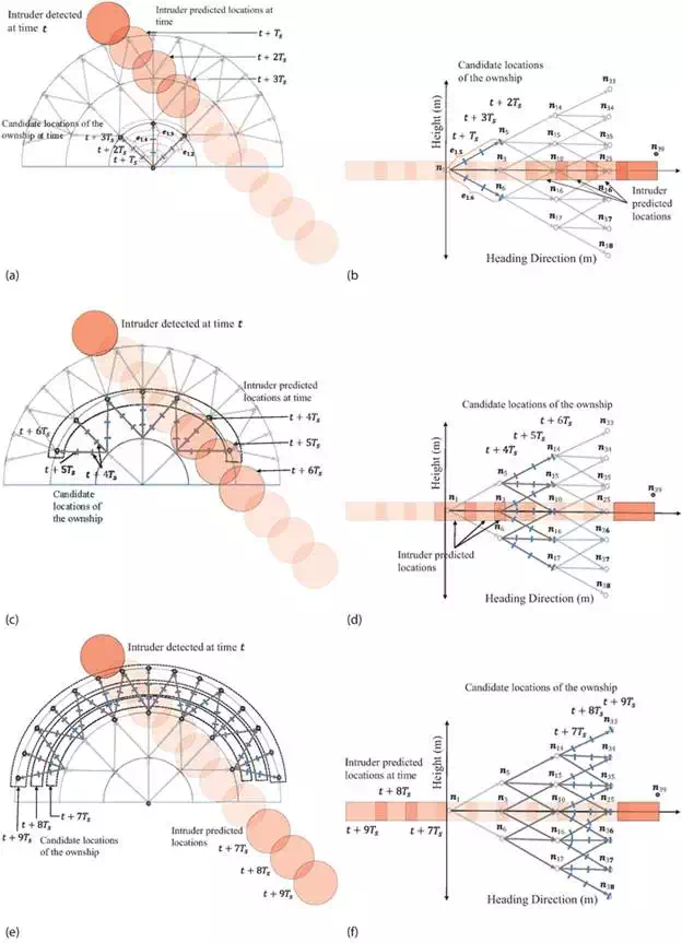
FIGURE 7.

Example illustrating the steps to compute the collision risk. In this example, we have k= 3 and m= 3. (a) Top view: predicted locations of intruder (less transparent circles), and candidate locations of ownship; (b) side view: predicted locations of intruder (less transparent rectangles), and candidate locations of ownship; (c) predicted locations of intruder and candidate locations of ownship over time window (t + 4Ts, t + 6Ts); (d) time window (t + 4Ts, t + 6Ts); (e) time window (t + 7Ts, t + 9Ts); (f) time window (t + 7Ts, t + 9Ts).

To provide an increased level of robustness, an additional threat cost is added to penalize edges close to the propagated locations of the intruder even if they are not within the collision volume. At each discrete time instant, we compute the distances from the candidate locations of the ownship to all the propagated locations of the intruders at that time instant. The cost of collision threat along each edge is then given by the sum of the reciprocal of the associated distances to each intruder

where d1,d2d1,d2, and d3d3 are given by

and the total collision risk cost associated with the iith edge with regard to all intruders is given by

For example, the edges e1,2, e1,3, e1,4, e1,5 and e1,6 shown in Figure 7a are not intersecting with the propagated collision volume locations over the first-time interval, yet they will be penalized based on their distances to the predicated locations of the intruder according to Eq. (15). Note that edge e1,2 will have greater cost as it is the closest to the intruder among other candidate edges.

Another objective of a path planning algorithm is to minimize the deviation from the original path, that is, the path the ownship was following before it detected a collision. Generally, the path is defined as an ordered sequence of waypoints W=w1,w2,⋯.wf  where wi=(wn,i,we,i,wd,i)T∈R3 is the north-east-down location of the iith waypoint in a globally known NED reference frame. The transformation from the global frame to the local-level frame is given by

where

where ψoψo is the heading angle of the ownship. Let wsws be the location waypoint of the ownship at the current time instant tt and wf∈W be the next waypoint the ownship is required to follow. Assuming a straight-line segment between the waypoints wsws and wfwf, then any point on this segment can be described as L(ϱ)=(1−ϱ)ws+ρwf where ϱ∈[0,1] and the minimum distance between an arbitrary node nini in GG can be expressed by

where

And

Then, the cost that penalizes the deviation of an edge in GG from the nominal path is given by

If small UASs are to be integrated seamlessly alongside manned aircraft, they may require to follow right-of-way rules. Therefore, an additional cost can be also added to penalize edges that violate right-of-way rules. In addition, this cost can be used to favor edges in the horizontal plane over those in the vertical plane. Since the positive direction of the yy-axis in the local-level frame is the right-wing direction, it is convenient to define right and left maneuvers as the positive and the negative directions along the right-wing axis, respectively. Let e→i≜ni+1−ni be the direction vector associated with the edge ei,i+1 in GG, where ni≜(xi,yi,zi)T∈R3 is the location of iith node in the local-level reference frame. Let the direction vector e→i be expressed as e→i=(eix,eiyeiz)T∈R3. We define E≜(eix,L,R,eiz)T∈R4, where eix and eiz are the x and the z components of e→i. The y-component of e→i is decomposed into two components: left L and right R, that are defined by

If we define the maneuvering design matrix to be J=diag([0,cL,cR,cz])J=diag0cLcRcz, then the maneuvering cost associated with each edge is given by

The costs cLcL and cRcR allow the designer to place more or less cost on the left or right edges. Similarly, cz allows the designer to penalize vertical maneuvers. Multiple values of these cost parameters may be saved in a look-up table, and the collision avoidance algorithm choses the appropriate value based on the geometry of the encounter.

The overall cost for traveling along an edge comes from the weighted sum of all costs given as

where k1, k2, and k3 are positive design parameters that allow the designer to place weight on collision risk or deviation from path or maneuvering preferences depending on the encounter scenario. Once the cost is assigned to each edge in G, then a graph-search method can be used to find the least cost path from a predefined start point to the destination point. In this work, we have used Dijkstra’s algorithm.

Dijkstra’s algorithm solves the problem of shortest path in a directed graph in polynomial time given that there are not any negative weights assigned to the edges. The main idea in Dijkstra’s algorithm is to generate the nodes in the order of increasing value of the cost to reach them. It starts by assigning some initial values for the distances from the start node and to every other node in the graph. It operates in steps, where at each step, the algorithm updates the cost values of the edges. At each step, the least cost from one node to another node is determined and saved such that all nodes that can be reached from the start node are labeled with cost from the start node. The algorithm stops either when the node set is empty or when every node is examined exactly once. A naive implementation of Dijkstra’s algorithm runs in a total time complexity of O(|N|2). However, with suitable data structure implementation, the overall time complexity can be reduced to O(|E|+|N|log2|N|) .

The local-level path planning algorithm generates an ordered sequence of waypoints Wc=wc1,wc2,⋯,wci. Then, these waypoints are transformed from the relative reference frame to the global coordinate frame and added to the original waypoints path W. When the ownship is avoiding a potential collision, the avoidance waypoints overwrite some or all of the original waypoints. Next, a path manager is required to follow the waypoints path and a smoother to make the generated path flyable by the ownship. One possible approach to follow waypoints path is to transit when the ownship enters a ball around the waypoint WiWi or a better strategy is to use the half-plane switching criteria that is not sensitive to tracking error . Flyable or smoothed transition between the waypoints can be achieved by implementing the fillet maneuver or using Dubins paths.

Simulation results

To demonstrate the performance of the proposed path planning algorithm, we simulate an encounter scenario similar to the planner geometry shown in Figure 8. The aircraft dynamics are simulated using a simplified model that captures the flight characteristics of an autopilot-controlled UAS. The kinematic guidance model that we considered assumes that the autopilot controls airspeed, va, altitude, h, and heading angle, ψ. Under zero-wind conditions, the corresponding equations of motion are given by

where pn, pe are the north-east position of the aircraft. The inputs are the commanded altitude, hchc, the commanded airspeed, vcavac, and the commanded roll angel, φcφc. The parameters bv, bφ, bh, and bḣ b are positive constants that depend on the implementation of the autopilot and the state estimation scheme. For further analysis on the kinematic and dynamic guidance models for UAS, we refer the interested reader to. In the following simulation, the ownship starts at (0,0,−200)T in the NED coordinate system, with an initial heading of 0 deg. measured from north and follows a straight-line path at a constant speed of 22 m/s to reach the next waypoint located at (1500,0,−200)T. The encounter geometry includes three intruders flying at different altitudes: the first is approaching head-on, the second is converging from the right, and the third is overtaking from the left. We chose the intruders’s speed similar to the known cruise speed of ScanEagle UAS, Cessna SkyHawk 172R, and Raven RQ-11B UAS. The speed of the intruders is 41, 65, and 22 m/s, respectively. In addition, the intruders are assumed to fly at a constant speed the entire simulation period. As shown in Figure 8, the initial locations of intruders in the NED coordinate system are (−25,1000,−225)T, (500,1000,−180)T, and (25,−500,−200)T respectively, with initial heading of 180, −90, and 0°, respectively.

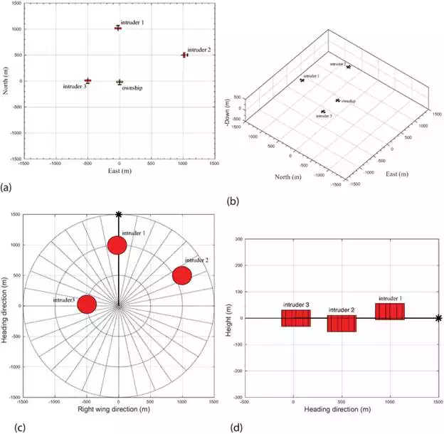
FIGURE 8.

Encounter geometry for the ownship and three intruders at tt = 0.1 s. (a) Overhead view of initial locations of aircraft; (b) 3D view of initial locations of aircraft; (c) overhead view of reference frame; (d) side view of relative reference frame.

In the following simulation, our choice of the collision volume is a cylinder of radius ds = 152.4 m (500 ft) and height hs = 61 m (200 ft) centered on each of the intruders. A collision incident occurs when the horizontal relative range and altitude to the ownship are simultaneously below horizontal and vertical minimum safe distances ds and hs/2. We assume that there exists a sensor and tracking system that provides the states of the detected intruders. However, not every aircraft that is observed by the sensing system presents a collision threat. Therefore, we implemented a geometric-based collision detection algorithm to determine whether an approaching intruder aircraft is on a collision course. The collision detection approach is beyond the scope of this work, and we refer the interested reader to.

At the beginning of simulation, the predicted relative range and altitude at the closest point of approach (CPA) are shown in Table 1. Imminent collisions are expected to occur with the first and second intruders as their relative range and altitude with respect to the ownship are below the defined horizontal and vertical safe distances. The time remaining to the closest point of approach tCPAtCPA with respect to the first and second intruders is 15.77 and 16.56 s, respectively. The scenario requires that the ownship plans and executes an avoidance maneuver well before the tCPA. This example demonstrates the need for an efficient and computationally fast avoidance planning algorithm. Table 2 shows the total time required to run the avoidance algorithm, and the maximum and average time required to execute one cycle. The results show that the proposed algorithm takes a significantly reduced time in computation with an average and maximum time to execute one cycle of the code of 20 ms and 0.1326 s, respectively, and a total time of 0.3703 s to resolve the collision conflict.

Intruder	∥pr(tCPA)∥ (m)	|prz(tCPA)| (m)	tCPA (s)
1	24.90	25	15.77
2	141.33	20	16.56
3	437.14	4361.07	1982.25

TABLE 1.

Relative range and altitude, and the time remaining to the closest point of approach.

Total run time (s)	Max. run time (one cycle) (s)	Average run time (one cycle) (s)
0.3703	0.1326	0.0206

TABLE 2.

Collision avoidance algorithm run time.

Figure 9 shows the planned avoidance path by the ownship. These results show that the avoidance path safely maneuvers the ownship without any collisions with the intruders. In addition, the ownship should plan an avoidance maneuver that does not lead to a collision with intruders that were not on a collision course initially such as the case with the third intruder. Initially, the third intruder and the ownship are flying on near parallel courses. The relative range and altitude at CPA with respect to the third intruder are 437.14 and 4361.07 m, respectively, and the time remaining to the CPA is 1982.25 s. Obviously, both aircrafts are not on a collision course. However, the third intruder is descending and changing its heading toward the ownship. The path planner, however, accounts for predicted locations of the detected intruder over the look-ahead time window, allowing the ownship to maintain a safe distance from the third intruder. This example demonstrates that the proposed path planner can handle unanticipated maneuvering intruders. Once collisions are resolved the path planner returns the ownship to the next waypoint of its initial path.

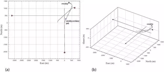
FIGURE 9.

Avoidance path followed by the ownship and path tracks of the intruders at tt = 75 s. (a) Overhead view of avoidance path and (b) 3D view of of avoidance path.

The relative range between the ownship and the intruders is shown in Figure 10. The results show that no collisions have occurred, and that the ownship successfully planned an avoidance maneuver. The avoidance planner ensures that when the relative horizontal range is less than dsds, the relative altitude is greater than hs/2hs/2. For example, as shown in Figure 10b, the relative range to the first intruder over time interval [16.2, 18] s is below dsds. However, over the same time interval, the relative altitude is above hs/2hs/2.

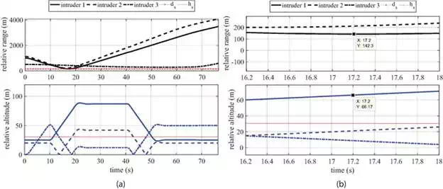
FIGURE 10.

Relative horizontal range and altitude between the ownship and intruders. (a) Horizontal range and relative altitude to intruders and (b) a close up view of Figure 10a.

Another important aspect to evaluate the performance of the proposed algorithm is its ability to reduce the length of the avoidance path while avoiding the intruders. This is important because it reduces the amount of deviation from the original path and ultimately the flight time, which is of critical importance for the small UAS with limited power resources. Table 3 shows that the length of the avoidance paths is fairly acceptable compared to the initial path length.

Scenario number	Initial path length (m)	Avoidance path length (m)
1	1500	1955

TABLE 3.

Length of the avoidance path.

Conclusions

In this chapter, we have presented a path planning approach suitable for small UAS. We have developed a collision avoidance logic using an ownship-centered coordinate system. The technique builds a maneuver graph in the local-level frame and use Dijkstra’s algorithm to find the path with the least cost.

A key feature of the proposed approach is that the future motion of the ownship is constrained to follow nodes on the map that are spaced by a constant time. Since the path is represented using waypoints that are at fixed time instants, it is easy to determine roughly where the ownship will be at any given time. This timing information is used when assigning cost to edges to better plan paths and prevent collisions.

An advantage of this approach is that collision avoidance is inherently a local phenomenon and can be more naturally represented in local coordinates than global coordinates. In addition, the algorithm accounts for multiple intruders and unanticipated maneuvering in various encounter scenarios. The proposed algorithm runs in near real time in Matlab. Considering the small runtime shown in the simulation results, we expect that implementing these algorithms in a compiled language, such as C or C++, will show that real-time execution is feasible using hardware. That makes the proposed approach a tractable solution in particular for small UAS.

An important step forward to move toward a deployable UAS is to test and evaluate the performance of the close-loop of sensor, tracker, collision detection, path planning, and collision avoidance. Practically, the deployment of any UAS requires a lengthy and comprehensive development process followed by a rigorous certification process and further analysis including using higher fidelity models of encounter airspace, representative number of simulations, and hardware-in-the-loop simulation. Unlike existing collision manned aviation collision detection and avoidance systems, an encounter model cannot be constructed solely from observed data, as UASs are not yet integrated in the airspace system and good data do not exist. An interesting research problem would be to design encounter models similar to those developed to support the evaluation and certification of manned aviation traffic alert and collision avoidance system (TCAS).