NATURAL WATER DRIVE

Natural water drive, as distinct from water injection, has already been qualitatively described, in Chapter 1, sec. 7, in connection with the gas material balance equation. The same principles apply when including the water influx in the general hydrocarbon reservoir material balance, equ. (3.7). A drop in the reservoir pressure, due to the production of fluids, causes the aquifer water to expand and flow into the reservoir. Applying the compressibility definition to the aquifer, then

in which the total aquifer compressibility is the direct sum of the water and pore compressibilities since the pore space is entirely saturated with water. The sum of cw and cf is usually very small, say 10-5/psi, therefore, unless the volume of water Wi is very large the influx into the reservoir will be relatively small and its influence as a drive mechanism will be negligible. If the aquifer is large, however, equ. (3.25) will be inadequate to describe the water influx. This is because the equation implies that the pressure drop ∆p, which is in fact the pressure drop at the reservoir boundary, is instantaneously transmitted throughout the aquifer. This will be a reasonable assumption only if the dimensions of the aquifer are of the same order of magnitude as the reservoir itself. For a very large aquifer there will be a time lag between the pressure change in the reservoir and the full response of the aquifer.

In this respect natural water drive is time dependent. If the reservoir fluids are produced too quickly, the aquifer will never have a chance to "catch up" and therefore the water influx, and hence the degree of pressure maintenance, will be smaller than if the reservoir were produced at a lower rate. To account for this time dependence in water influx calculations requires a knowledge of fluid flow equations and the subject will therefore be deferred until Chapter 9, in which a full description of the phenomenon is provided. For the moment, the simple equation (3.25) will be used to illustrate the influence of water influx in the material balance.

Using the technique of Havlena and Odeh (assuming that Bw = 1), the full material balance can be expressed as

in which the term Ef,w, equ. (3.11), can frequently be neglected when dealing with a water influx. This is not only for the usual reason that the water and pore compressibilities are small but also because a water influx helps to maintain the reservoir pressure and therefore, the ∆p appearing in the Ef,w term is reduced. This is a point which should be checked at the start of any material balance calculation (refer exercise 9.2). If, in addition, the reservoir has no initial gascap then equ. (3.12) can be reduced to

In attempting to use this equation to match the production and pressure history of a reservoir, the greatest uncertainty is always the determination of the water influx We. In fact, in order to calculate the influx the engineer is confronted with what is inherently the greatest uncertainty in the whole subject of reservoir engineering. The reason is that the calculation of We requires a mathematical model which itself relies on the knowledge of aquifer properties. These, however, are seldom measured since wells are not deliberately drilled into the aquifer to obtain such information. For instance, suppose the influx could be described using the simple model presented as equ. (3.25). Then, if the aquifer shape is radial, the water influx can be calculated as

in which re and ro are the radii of the aquifer and reservoir, respectively, and f is the fractional encroachment angle which is either Θ/2π or Θ/360°, depending on whether Θ is expressed in radians or degrees. It should be realised that the only term in equ. (3.27) which is known with any degree of certainty is π! The remaining terms all carry a high degree of uncertainty. For instance, what is the correct value of re? Is the aquifer continuous for 20 kilometers or is it truncated by faulting? What is the correct value of h, the average thickness of the aquifer or φ, the porosity? These can only be estimated, based on the values determined in the oil reservoir. For such reasons, building a correct aquifer model to match the production and pressure data of the reservoir is always done on a "try it and see" basis and even when a satisfactory model has been achieved it is seldom if ever, unique. Therefore, the most appropriate way of applying equ. (3.26) is by expressing it as

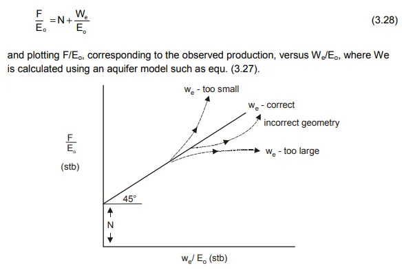
Once a satisfactory aquifer model has been obtained by history matching, the same model can hopefully be used in predicting reservoir performance for any scheduled offtake policy. As already mentioned, however, there are so many uncertainties involved that the aquifer model is hardly ever unique and its validity should be continually checked as fresh production and pressure data become available.