THE SONIC OR ACOUSTIC LOG

Introduction

Wave Types

The tool measures the time it takes for a pulse of “sound” (i.e., and elastic wave) to travel from a transmitter to a receiver, which are both mounted on the tool. The transmitted pulse is very short and of high amplitude. This travels through the rock in various different forms while undergoing dispersion (spreading of the wave energy in time and space) and attenuation (loss of energy through absorption of energy by the formations). When the sound energy arrives at the receiver, having passed through the rock, it does so at different times in the form of different types of wave. This is because the different types of wave travel with different velocities in the rock or take different pathways to the receiver. Figure 16.1 shows a typical received train of waves. The transmitter fires at t = 0. It is not shown in the figure because it is masked from the received information by switching the receiver off for the short duration during which the pulse is transmitted. This is done to ensure that the received information is not too complicated, and to protect the sensitive receiver from the high amplitude pulse. After some time the first type of wave arrives. This is the compressional or longitudinal or pressure wave (P-wave). It is usually the fastest wave, and has a small amplitude. The next wave, usually, to arrive is the transverse or shear wave (S- wave). This is slower than the P-wave, but usually has a higher amplitude. The shear wave cannot propagate in fluids, as fluids do not behave elastically under shear deformation. These are the most important two waves. After them come Rayleigh waves, Stoneley waves, and mud waves. The first two of these waves are associated with energy moving along the borehole wall, and the last is a pressure wave that travels through the mud in the borehole. They can be high amplitude, but always arrive after the main waves have arrived and are usually masked out of the data. There may also be unwanted Pwaves and S-waves that travel through the body of the tool, but these are minimized by good tool design by (i) reducing their received amplitude by arranging damping along the tool, and (ii) delaying their arrival until the P-wave and S-wave have arrived by ensuring that the pathway along the tool is a long and complex one. The data of interest is the time taken for the P-wave to travel from the transmitter to the receiver. This is measured by circuitry that starts timing at the pulse transmission and has a threshold on the receiver. When the first P-wave arrival appears the threshold is exceeded and the timer stops. Clearly the threshold needs to be high enough so that random noise in the signal dies not trigger the circuit, but low enough to ensure that the P-wave arrival is accurately timed.

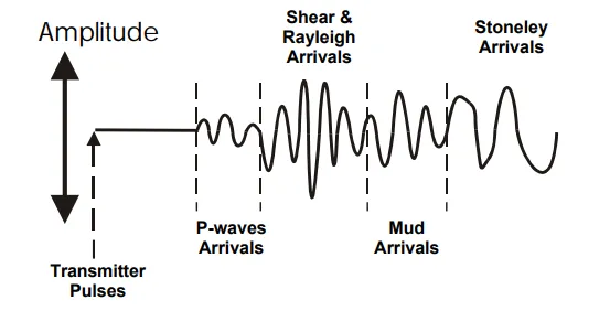
The geophysical wavetrain received by a sonic log

There are complex tools that make use of both P-waves and S-waves, and some that record the full wave train (full waveform logs). However, for the simple sonic log that we are interested in, only the first arrival of the P-wave is of interest. The time between the transmission of the pulse and the reception of the first arrival P-wave is the one-way time between the transmitter and the receiver. If one knows the distance between the transmitter (Tx) and the receiver (Rx), the velocity of the wave in the formation opposite to the tool can be found. In practice the sonic log data is not presented as a travel time, because different tools have different Tx-Rx spacings, so there would be an ambiguity. Nor is the data presented as a velocity. The data is presented as a slowness or the travel time per foot traveled through the formation, which is called delta t (Dt or DT), and is usually measured in ms/ft. Hence we can write a conversion equation between velocity and slowness: