Gridding and Well Modelling Learning Objectives

*Understand and be able to describe the basic idea of gridding and of spatial and temporal discretization

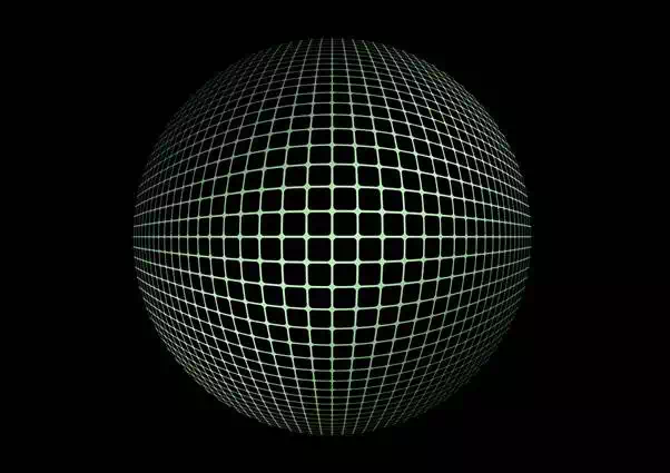
Gridding is the process of dividing the entire reservoir up into small spatial blocks which then compromise the units on which the numerical block to block flow calculations are performed. This is known more formally as spatial discretization.

There is also the process of dividing up blocks into time steps (Δt) and this is referred to as temporal discretization.

*Be aware of all the main types of grid in 1D, 2D and 3D used in reservoir simulation and be able to describe examples of where it is most appropriate to use the different grid types.

The main types of grids in the following dimensions are:

1D – Linear

We can use this to model a 1D Buckley-Leverett type water displacement calculations (x-direction) or for single column vertical displacements (z-direction).

2D – Cartesian Grids

2D cross-sectional can be used to study vertical sweep efficiency in a heterogeneous layered system, calculate water/oil displacements in a geostatistically generated cross-section, generate pseudo relative permeabilities.

2D – Areal

2D areal (x/y grids) maybe be used to calculate areal sweep efficiencies in a waterflood oor a gas flood, to examine the stability of a near miscible gas injection within a heterogeneous reservoir layer, examine the benefits of infill drilling in an areal pattern flood.

3D – Cartesian Grid

(x/y/z grids) are the most versatile but not appropriate for all flow conditions in a reservoir. Close to the wellbore flow patterns are more radial in nature and so 3D Cartesian grid would poorly simulate this.

*Be able to give a short description with simple diagrams of the phenomena of numerical dispersion and grid orientation and to explain how these numerical problems can be overcome.

Numerical dispersion is the error that arises when we use a grid block approximation for solving flow equations. There is usually a trade-off between accuracy and computational cost.

*Be familiar with more sophisticated issues in gridding such as the use of local grid refinement (LGR), distorted, PEBI and corner point grids.

Local Grid Refinement

Local grid refinement is required in areas where there is a significant change in reservoir properties over a small area. This is necessary in order to more accurately simulate real world conditions. In sections where the changes are small over large areas we can have a coarse grid which will save computational power.

Distorted

Distorted grids get their name from the irregular shape of the grid blocks and are formed by adhering to the non-uniform shape of the reservoir.

PEBI – Perpendicular Bisector

PEBI grids are used primarily to model faults in reservoirs. In the PEBI grid the chosen grid points are blocked off into volumes using a geometrical construction.

Corner Point Geometry

It can be tedious using corner point geometry as the grid is built up by specifying all eight corners of every block. Corner point geometry can be a time consuming process when modelling complex reservoirs, it can be used to model a major fault in between aquifer and reservoir.

*Given a specific task for reservoir simulation, the student should be able to select the most appropriate grid dimension (1D, 2D, 3D) and geometry/structure (Cartesian, r/z, corner point etc.).

All of these conditions are depend entirely upon the problem we are trying to solve. There is no one size fits all solution. But here are some examples:

· A 2D x/z cross-sectional model (with dip if necessary) may be used to study the effects of vertical heterogeneity – layering as an example – on the sweep efficiency or water breakthrough time.

· For a near well coning example, an r/z grid is more appropriate – it more closely reflects the radial nature of the problem

· 2D x/z grids are also used to generate pseudo relative permeabilities for use in 2D areal models

· Full field simulations require use of 3D Cartesian grids with grid mesh refinement in the appropriate locations

*Be able to discuss the issues of grid fineness/coarseness (i.e. how many grid blocks do we need to use) in terms of some examples of what can happen if an inappropriate number of grid blocks are used in a reservoir simulation calculation.

In order to determine the appropriate number of grid blocks we can perform simulations and continually refine the mesh until we see the results converging. When the results no longer change with a refining grid mesh, we can conclude that the calculation is converged and is probably reliable.

If the grid is far from being converged, then comparisons between different sensitivity calculations may be masked by numerical errors.

*Be able to describe the basic ideas behind streamline simulation and to compare it with conventional reservoir simulation in terms of its advantages and disadvantages

Streamline simulation counters the effect of numerical dispersion and generates a more accurate transport calculation. Typically, the process begins by calculating the pressure distribution in a given permeability field by solving a conventional pressure equation. From this the iso-potentials are determined (pressure contours) and the gradient of the pressures locally perpendicular to the iso-potentials are the streamlines. Determining velocity from Darcy’s law it is possible to solve for how far the saturation front moves along the streamline. The advance of the streamline can be calculated with reliable accuracy avoiding the issue of block to block numerical dispersion.

*Be familiar with the different types of average used for single phase average kA, two phase relative permeabilities (k_rp) and for µ_p and B_p (p = o, w, g phase) when calculating the block to block flows (Q_p) in a reservoir simulator.

The appropriate average kA to use when modelling single phase permeability is the harmonic average weighted by the grid block sizes. The harmonic average gives much more weighting to the lower permeability value. If the grid sizes are equal, this reduces to the exact harmonic average k_H. It is much more affected by lower permeability, since if one of the permeabilities was zero then the flow would be zero, no matter how large the other permeabilities were.

Averaging of the two phase mobility term λp – we separate the relative permeability term from the viscosity and consider them separately as λ_p, µ_p and B_p.

The physically correct value of relative permeability is the upstream value.

*Be able to describe the physical justification for using the upstream value of two phase relative permeabilities when calculating the block to block flows (Q_p) in a reservoir simulator.

*Understand the origin of all the pressure drops that are experienced by the reservoir fluids from deep in the reservoir, through to the wellbore and then to the surface facilities and beyond.

The origin of pressure drops can be from as follows:

· Formation to wellbore flow – where fluids form a drainage radius r_e at pressure P_eto the wellbore (this can also be thought of as bottom hole flowing pressure)

· Pressure drop that may occur along the completed region of the wellbore from the bottom of the well to the wellbore just at the top of the completed interval

· The pressure drop from the well at the top of the completed formation just above the reservoir to the wellhead. As fluid is being produced, the pressure drops in oil/water production and free gas may also appear. We can therefore have three phase flow in the well casing to the surface and this may need to be incorporated into the reservoir simulation model

· Pressure drops can also occur as the produced fluids flow from the wellhead through the surface equipment such as separators and various chokes.

*Know what a well model is and what productivity index (PI) is, including knowing the radial Darcy Law and how this gives a mathematical expression for PI for single phase flow (KNOW THE EXPRESSION FROM MEMORY)

Productivity Index is a measure of the ability of a well to produce. It is defined by the symbol J, the productivity index is the ratio of the total liquid flow rate to the pressure drawdown.

The productivity index is:

We can also manipulate the radial Darcy Law equation for a single phase flow to get the productivity index equation. We need to assume P = P_e at r_e. Once we make this assumption and rearrange the equation we get a value for PI:

*Be able to describe the main issues in relating the pressure in the reservoir, P_e, at some drainage radius, r_e, to an average grid block pressure and how this leads to the Peaceman formula (Δr = 0.2 Δx) which is then used to calculate PI.

Firstly, the relation between r_e and the block size (Δx, Δy)

If Δx = Δy → r_e ≈ 0.2Δx

If Δx ≠ Δy → r_e ≈ 0.14

Secondly, the relation between P_e and the average grid block pressure, P.

*Describe a well model for a multi layer system where there is two phase flow into the wellbore

Since all four layers may be producing both oil and water and each phase can be changing as the saturations and relative permeabilities change. There is also a gravitational potential that must be taken into account for each situation. There’s a few equations, refer to the text book page 37 to see them.

*Understand and be able to describe the various types of well constraint that can be applied e.g. injection volume constrained wells, well flowing pressure constraints and voidage replacement constraints.

A common well constraint is to fix the water injection rate at the injector with a limit on the well flowing pressure. A producer is then controlled by setting the bottom hole flowing pressure and then oil and water phase flows may then be calculated (Q_o and Q_w).