FLOW PROPERTIES OF FLUIDS

The fluid state

It is an everyday experience that all matter exists in either the fluid or the solid state. This also invariably applies under the physical circumstances of hydrocarbon production and technology. The different molecular structure of fluids and solids manifests itself in different macroscopic properties. From the point of view of this

book only those properties are of interest, which relate to the motion of fluids, or the conditions affecting this motion. In the fluid state molecules have great mobility;

translation, rotation and vibration are all allowed. In contrast to this, a solid is characterized by a restricted molecular mobility, only vibration and rotation about a fixed average position is possible. Fluids and solids behave differently under the action of external forces. A solid has tensile strength, while a fluid has none (except for viscoelastic materials). Fluids have no shape of their own, they always fill their container, adopting its shape. A fluid resists compressive forces only if it is kept in a container. Solids can withstand shearing stress up to their elastic limit, whereas fluids subjected to shearing stresses deform immediately and for as long as the stress is applied. The force of friction between two solids depends on the pressure which compresses the two surfaces; fluid friction is independent of the applied pressure. Between solids frictional forces can exist at rest, whereas in fluids shear stresses vanish in the hydrostatic state. Fluids are isotropic materials, in contrast to most solids. These differences in mechanical behavior help to define what is a fluid. A fluid is considered to be an isotropic material which deforms continuously under the influence of an applied external force. The characteristic form of fluid motion is that of flow, which is represented mathematically by a continuous transformation of three-dimensional Euclidean space into itself. Any fluid, no matter how viscous, will flow even under the slightest tangential stress. Tangential stresses between adjacent fluid particles are proportional to the rate of deformation and disappear when the flow ceases; remnant stresses cannot exist in fluids. A fluid may be either a liquid or a gas. Liquids are relative incompressible, whereas gases are highly compressible. Liquids have a constant density and volume (slightly dependent on temperature), gases tend to expand infinitely. A liquid can have a free surface at which the pressure is constant and equal to the gas or vapor pressure over it.

The molecules of gases are spaced far away from each other, and have a high translation energy. The kinetic energy of this molecular translation is much greater

than the energy of attraction between the molecules. The average distance between the molecules of a liquid is much smaller; the translation kinetic energy being lessthan the energy of attraction between the molecules. The distribution of the translation energy among the molecules of a liquid follows Maxwell’s distribution law. Certain molecules therefore may have enough kinetic energy to overcome the attraction of adjacent molecules. These molecules can thus escape from the liquid and form a vapor. Liquids, consequently, exert a vapor pressure which is the  pressure attained by the vapor when left in contact with its liquid until equilibrium is achieved at constant temperature. The vapor pressure is a function of temperature. The main difference between a gas and a vapor is that a gas cannot be liquefied by compression alone. For a vapor this is obviously possible. An essential difference between liquids and gases lies in their compressibility. Since liquids can only be compressed very slightly, even at very high pressures, they can be considered to be incompressible. Thus pressure becomes a simple mechanical variable and is no longer a thermodynamic variable. In this case mechanical and thermal processes may be considered separately. In contrast to the cases for a liquid, the density of a gas is strongly affected by changes in pressure and temperature. Since pressure now is a variable of the thermal state, mechanical and thermal processes must be considered simultaneously.

The continuum model of fluids

Like any other material a fluid is discrete at the microscopic level. The dimensions typically involved in engineering problems are however, much greater than

molecular distances. A mathematical description of fluid flow consequently require  that the actual molecular structure be replaced by a hypothetical continuous

medium, called the continuum. This continuum continuously occupies a threedimensional space, and can be infinitely subdivided while still preserving its original

properties. In the continuum model the actual material is replaced by continuous functions of physical quantities. The actual physical processes are represented

by the evolution of these continuous functions in space and time. This spatial- and time-evolution can be expressed by means of partial differential equations. The value of such a function at a certain point is obtained as an average value in the infinitesimal volume d V surrounding the point. The essential mathematical simplification of the continuum model is that this average value is, in the limiting case, assigned to the point itself. This infinitesimal fluid element of volume d V must contain a sufficient number of molecules to allow a statistical interpretation of the continuum. When the molecular dimensions are very small compared with any characteristic dimension of the flow system, the average values obtained in this fluid element may be considered as variables at a given point. This infinitesimal fluid element is called a fluid particle. This notion of a fluid particle is not to be confused with any particle of the molecular theory. To illustrate the limiting process by which the local continuum properties can be defined, consider a small volume A V surrounding a point P, the mass of fluid in AV is now Am. The ratio

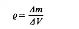
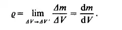
will asymptotically approach a certain limiting value, as AV becomes smaller. When A V has decreased to a certain value A V' striking random fluctuations begin

to appear since the number of molecules is too low to produce a statistically valid result. Thus the density is defined as

The limiting process is carried out only to A V instead of to zero. This approximation can never be valid when the characteristic dimensions of the fluid system are

but slightly larger than the molecular distances. The latter is the case when a fluid flows through very narrow capillaries, or in the rarefied atmosphere of highaltitude

flights.

Variables of state

If any material system is left alone for a sufficient length of time, it will achieve a state of equilibrium. In this equilibrium state all macroscopically measurable quantities are independent of time. Variables that depend only on the state of the system are called variables of state. The pressure p and the density e are obviously variables of the mechanical state of the system. The thermal state of the system can also be characterized by the pressure and density, but it is an experimental observation that the density of the system is not solely a function of its pressure; a third variable of state, the temperature T, must be considered. The relation between the variables of state can be expressed by the equation of state

In the equation of state, the density is often replaced by its reciprocal called the specific volume

In general it is not possible to express the equation of state in a simple analytic form. It can only be tabulated or plotted against the variables of state. It is obvious that an equation such as

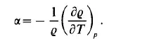
can be represented by a surface in the coordinate system 9, T, p. This surface of state consists of piecewise continuous surface parts, as shown in Fig. 1.1. It is

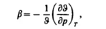
customary to plot this relation as projected onto any one of the three planes p- 9, p- T, or 9- T. In such a projection the third variable of state is treated as a parameter. The most common diagram of state is that of water as shown in Fig.1.2. Thus we obtain isothermal curves (isotherms) in the p, 9 plane, the isobars in the 9, T plane and the isochores in the p, T plane. The shape of the surface of state is characteristic of a particular material. Three partial derivatives of the equation of state determine three important properties of a material. The coefficient of thermal expansion is defined by the expression

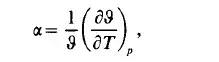
or, expressed in terms of the density:

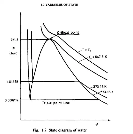
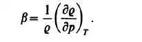
The isothermal compressibility is defined by the derivative

or, in terms of the density:

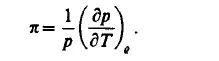
The isochoric pressure coefficient is obtained as

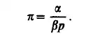
Since a, fl and II are interrelated through the variables of state, Eqs (1.5H1.9) can also be considered as expressions of the equation of state. The latter can then

be written as

In certain regions of the surface of state, the equations of state can be determined experimentally. Such a degenerated equation of state is the condition of incompressibility

The condition of incompressibility does not exclude the density varying with the temperature. Since many flows may be considered to be isothermal, the condition

of incompressibility merely signifies a constant density at a given temperature while a flow problem is being solved. Usually a reference density eo is given (generally

at 15 "C), from which the density at an arbitrary temperature can be obtained as

At constant temperature the variation in the density as a function of pressure can be expressed as

For gases at low pressures and remote from the two-phase boundary the equation of state of an ideal gas,

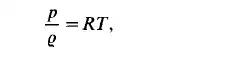
provides reasonable accuracy for engineering calculations. In this equations R is the gas constant with dimensions [J/kg "C]. More suitable to calculations in the field of petroleum engineering, where greater pressures are involved, is the modified equation of state:

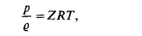
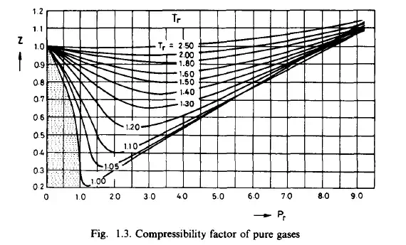
where Z is the dimensionless compressibility factor. This can be obtained from a diagram, where Z is plotted against the reduced pressure at constant values of

reduced temperature. The compressibility factor chart of Viswanath and Su is shown in Fig. 1.3. When the energy relations, i.e. the exchange of work and heat between a system and its surroundings are considered it seems to be necessary to define two further variables of state the internal energy E , and the enthalpy i. For a simple system E

and i are functions of any two of p , 9 and T. Thus the so-called caloric equation of state can be written

A specific material can be characterized by its equations of state. These equations cannot be deduced from thermodynamic principles; they are obtained experimentally.

For incompressible fluids and for perfect gases the caloric equations of

state are obtained in very simple form

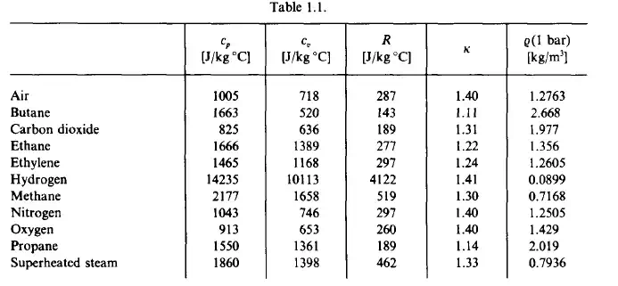
where c, and cp are the heat capacities at constant volume (or density) and at constant pressure. The relations between c, and cp are obtained in the form

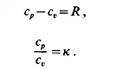
Both c,, cp, R and x are important material constants. They are tabulated in Table 1.1. Variables of state can be classified as either intensive or extensive variables.

Intensive variables are related to the points of a system, thus they are point functions. Velocity, pressure and temperature are typical intensive variables. Intensive

variables can relate to a finite region only if their distributions are uniform. In this case both the values of a variable relating to the whole region, and that relating

to a part of it must be the same. Extensive variables are related to a finite region of a system, thus they are set functions. The mass of the system is such an extensive variable, and so are the volume, momentum, energy, entropy, etc. Set functions are additive, for example the momentum of a certain body is equal to the sum of the momentums of its parts. Specific quantities such as density or specific enthalpy would seem to be intensive variables since their values vary from point to point in the manner of point functions. There is, however, an essential difference between such specific quan-

tities and real intensive variables. The specific quantities may be integrated over a region thus producing an extensive variable; for a real intensive variable such an

integration has no physical meaning. Intensive and extensive variables play different roles in physical processes. The state of a material system can be determined by as many extensive variables as there are types of interaction between the system and its surroundings. An interaction of certain type may induce either equilibrium or a process of change. A characteristic pair of intensive and extensive variables are associated with any interaction. The characteristic intensive variable is that one which is uniformly distributed at equilibrium. For instance, experimental observations show that thermal equilibrium can exist only if the temperature has a uniform distribution throughout the whole system. A homogeneous velocity distribution is associated with the condition of mechanical equilibrium. A system with a uniformly distributed velocity U is at rest in a coordinate system moving with the velocity U. Thus temperature and velocity have particular significance as the characteristic variables of thermal

and mechanical interaction. If the distribution of the characteristic intensive variable is not homogeneous, the equilibrium condition is terminated and certain processes are induced accompanied by changes in the extensive variables. These changes are directed so as to neutralize the inhomogeneity. Fluxes of extensive quantities may be convective, i.e. transferred by macroscopic motion, or conductive, i.e. transferred by molecular motion only. Conductive fluxes can be expressed by the product of a conductivity coefficient and the gradient of the characteristic intensive variable. These conductivity coefficients are important material properties.

Conductivity coefficients

In petroleum engineering the material systems considered may be in mechanical and thermal interaction with their surroundings. In the case of mechanical interaction

the stress is the conductive flux of momentum. This conductive momentum flux for one-dimensional motion is expressed as

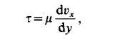
where T is the momentum conductively transferred across a unit area per unit time, dux/dy is the velocity gradient, and p is a coefficient of proportionality the dynamic

viscosity coefficient, usually called just the viscosity. The viscosity coefficient p is a characteristic property of fluids. Its value for a particular fluid may be a function of temperature, pressure and the shear rate. In the simplest case the viscosity coefficient is a function of the temperature only. For isothermal fluids the viscosity is then constant. If the viscosity is independent of the shear rate the fluid is called Newtonian. The viscosity of all Newtonian liquids decreases with increasing temperature at constant pressure. The viscosity of  gases increases with temperature at constant pressure. The viscosity of pure liquids depends strongly on the temperature, but is relative insensitive to pressure variations, At extremely high pressures (p- 1000 bar) the viscosity of a liquid increases remarkably with pressure. The viscosity of gases at

low pressures may be calculated based on kinetic theory. Above 8-10 bars the effect

of pressure becomes significant. In many hydrodynamic equations it is common to use the quotient of the viscosity divided by the density. This is the so-called

kinematic viscosity,

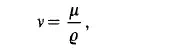
with the dimensions [m’/s]. Both the dynamic and kinematic viscosities of some common fluids are tabulated in Table 1.2. In the case of thermal interaction between a system and its surroundings the conductive flux of the internal energy for the one-dimensional case is given by

where q is the rate of flow of internal energy across a unit area per unit time, dT/dx the temperature gradient, and k is the thermal conductivity coefficient. Its dimensions

are w / m “C]. The thermal conductivity coefficient depends on the temperature, and for gases to a certain degree on the pressure.