Gravity data interpretation
The interpretation of gravity data could be only a simple qualitative analysis in a way: “Look, there is a sharp local decrease of gravity, this could be a cave!” Or a more complex quantitative analysis, where, based on the qualitative assignment, we try to somehow model the subsurface. In this respect we have to bear in mind that the interpretation (inversion) of geophysical data is non-unique.
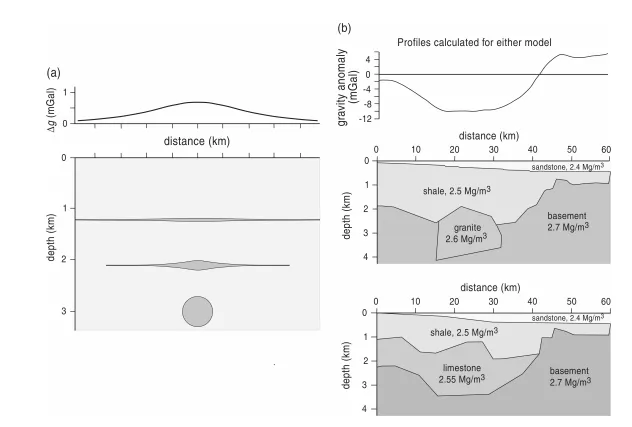
In gravity prospection not only that different bodies could have similar anomalies (cf. figures 2.8 and 2.9) they can also produce exactly the same anomaly (Fig. 2.16). The nonuniqueness is inherent to gravity data and could not be overcome e.g. by adding more gravity data.
The only way how to get sound and reliable interpretation is to include an a priori geological knowledge and, if possible, also data from another geophysical methods. Another aspect is that the measured anomaly depends solely on the density contrast (difference) between the bodies. Hence a sphere with the density of 2.3 g/cm3 surrounded by the rocks with a density 2.5 g/cm3 will produce exactly the same anomaly as a sphere with the density of 2.5 g/cm3 surrounded by the rocks with a density 2.7 g/cm3 .
In a similar manner a half slab on one side of a fault with a positive density contrast could produce the same anomaly as a half slab on the other side with a negative density contrast.


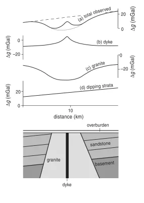
As we have already seen in the section 2.5, simple rules for estimation of depth of some simple bodies could be derived. There are some more in the figure 2.18. These rules are useful for estimating initial parameters for further modelling. Building models from simple geometrical bodies is easy, however, one can easily see that not all the geological bodies could be easily approximated by them. Therefore, another modelling techniques were developed.
One of these is building the models from polygonal bodies with arbitrary number of corners (Figs. 2.16b, 2.19). There are formulas for computing gravity effects of such bodies, often based on the original Talwani’s algorithm developed in late fifties (Talwani 1959). The modelled bodies are usually 2D (infinite in the y direction) or 2.5D (bodies have limited length in the y direction). However, equations for 3D modelling are also available. The advantage of this (polygonal) approach is in fact that the computations are fast and memory cheap and can be easily run on any of current computers.
There are number of such computer programs available here and there (e.g. Cooper 2012, Fig. 2.19). The usual approach is to build an initial model estimated according to the measured gravity data and geological evidence and then using either a trial and error technique and to some extent also with automated inversion procedures we try to match the measured and modelled gravity curves. Due to the nonuniqueness of the gravity data, there are, unlike to some other geophysical methods, no “black-box” automated inversions.
Currently, it is not possible to put data into some computer program, press a button and get the result. Although there are some attempts to achieve this. Another approach is to divide the model into regular cells and assign each cell some density value (e.g. Snopek and Casten 2006). The cells are usually cubes, but any geometrical representation is possible. This kind of discretisation is common to many geophysical methods. The advantage is that arbitrarily complex models could be achieved.
The drawback – the number of cells (and hence also the parameters) very quickly arises, mainly for the 3D case, and the computing gravity effect of such model is (computationally) very expensive.