Fundamentals of Optical Information Processing

Optical information processing is based on the idea of using all the properties of speed and parallelism of the light in order to process the information at high-data rate. The information is in the form of an optical signal or image. The inherent parallel processing was often highlighted as one of the key advantage of optical processing compared to electronic processing using computers that are mostly serial. Therefore, optics has an important potential for processing large amount of data in real time.

The Fourier transform property of a lens is the basis of optical computing. When using coherent light, a lens performs in its back focal plane the Fourier transform of a 2D transparency located in its front focal plane. The exact Fourier transform with the amplitude and the phase is computed in an analog way by the lens. All the demonstrations can be found in a book published in 1968 by Goodman and this book is still a reference in the field. The well-known generic architecture of optical processors and the architectures of the optical correlators will be presented successively.

Optical Processor Architecture

The architecture of a generic optical processor for information processing is given in Figure 1.

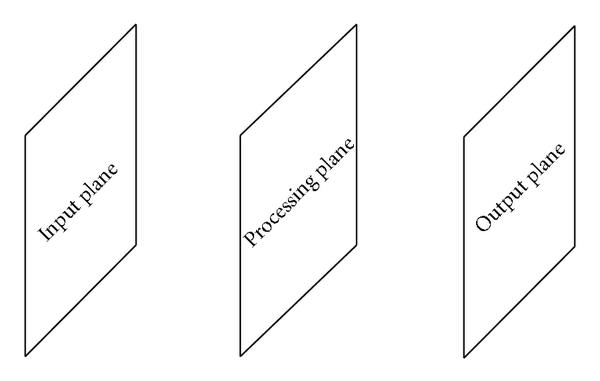
Figure 1

Architecture of an optical processor.

The processor is composed by three planes: the input plane, the processing plane, and the output plane.

The data to be processed are displayed in the input plane, most of the time this plane will implement an electrical to optical conversion. A Spatial Light Modulator (SLM) performs this conversion. The input signal can be 1D or 2D. An acousto-optic cell is often used in the case of a 1D input signal and 2D SLMs for 2D signals. The different types of 2D SLMs will be described later. In the early years, due to the absence of SLMs, the input plane consisted of a fixed slide. Therefore the principles and the potential of optical processors could be demonstrated but no real-time applications were possible, making the processor most of the time useless for real life applications.

The processing plane can be composed of lenses, holograms (optically recorded or computer generated) or nonlinear components. This is the heart of the processing, and in most optical processors, this part can be performed at the speed of the light.

A photodetector, a photodetector array or a camera composes the output plane where the results of the processing are detected.

Figure 1 shows clearly that the speed of the whole process is limited by the speed of its slowest component that is most of the time the input plane SLM, since the majority of them are operating at the video rate. The SLM is a key component for the development of practical optical processors, but unfortunately also one of their weakest components. Indeed, the poor performance and high cost of SLMs have delayed the fabrication of an optical processor for real-time applications.

Optical Processors Classical Architectures

At the beginning, real-time pattern recognition was seen as one of the most promising application of optical processors and therefore the following two architectures of optical correlators were proposed.

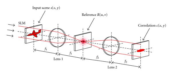
Figure 2(a) shows the basic correlator called 4-f since the distance between the input plane and the output plane is four times the focal length of the lenses. This very simple architecture is based on the work of Maréchal and Croce in 1953 on spatial filtering and was developed during the following years by several authors .

(a)

(b)

(c)

(a)
(b)
(c)

Figure 2

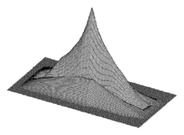
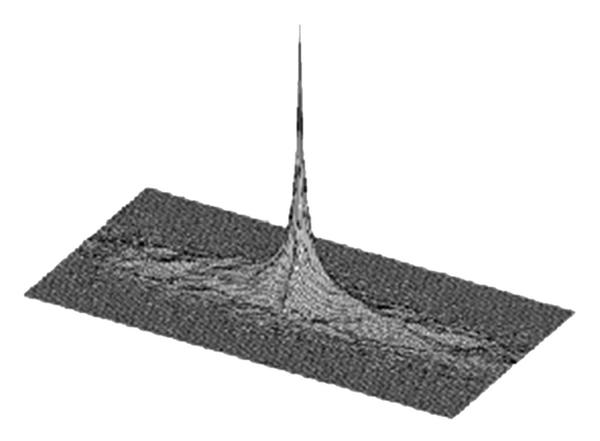
Basic 4-f correlator: (a) Optical setup. (b) Autocorrelation peak for a matched filter. (c) Autocorrelation peak for a phase only filter.

The input scene is displayed in the input plane which Fourier transform is performed by Lens 1. The complex conjugated of the Fourier transform of the reference is placed in the Fourier plane and therefore multiplied by the Fourier transform of the input scene. Lens 2 performs a second Fourier transform that gives in the output plane the correlation between the input scene and the reference. Implementing a complex filter with the Fourier transform of the reference was the main challenge of this set-up, and Vander Lugt proposed in 1964 to use a Fourier hologram of the reference as a filter . Figures 2(b) and 2(c) show respectively, the output correlation peak for an autocorrelation when the correlation filter is a matched filter and when it is a phase only filter .

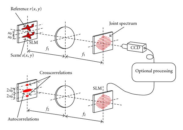
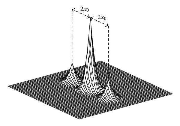
In 1966, Weaver and Goodman [14] presented another optical correlator architecture, the joint transform correlator (JTC) that is represented by Figure 3(a). The two images, the reference  and the scene  are placed side by side in the input plane that is Fourier transformed by the first lens. The intensity of the joint spectrum is detected and then its Fourier transform is performed. This second Fourier transform is composed by several terms including the crosscorrelations between the scene and the reference. Using a SLM this Fourier transform can be implemented optically as shown on Figure 3(a). Figure 3(b) shows the output plane of the JTC when the reference and the scene are identical . Only the two crosscorrelation peaks are of interest. To have a purely optical processor, the CCD camera can be replaced by an optical component such as an optically addressed SLM or a photorefractive crystal. One of the advantages of the JTC is that no correlation filter has to be computed, therefore the JTC is the ideal architecture for real-time applications such as target tracking where the reference has to be updated at a high-data rate.

(a)

(b)

(a)
(b)

Figure 3

Joint transform correlator (JTC): (a) Optical setup. (b) Output plane of the JTC.

Figures 2 and 3 represent coherent optical processors. Incoherent optical processors were also proposed: the information is not carried by complex wave amplitudes but by wave intensities. Incoherent processors are not sensitive to the phase variations in the input plane and they exhibit no coherent noise. However, the nonnegative real value of the information imposes to use various tricks for the implementation of some signal processing applications .

Linear optical processing can be decomposed into space-invariant operations such as correlation and convolution or space-variant operations such as coordinates transforms [17] and Hough transform. Nonlinear processing can also be implemented optically such as logarithm transformation, thresholding or analog to digital conversion .