Analysis of Classic Ethernet

How much time does Ethernet “waste” on collisions? A paradoxical attribute of Ethernet is that raising the transmission-attempt rate on a busy segment can reduce the actual throughput. More transmission attempts can lead to longer contention intervals between packets, as senders use the transmission backoff algorithm to attempt to acquire the channel. What effective throughput can be achieved?

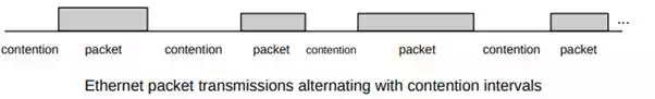
It is convenient to refer to the time between packet transmissions as the contention interval even if there is no actual contention, that is, even if the network is idle; we cannot tell if stations are not transmitting because they have nothing to send, or if they are simply waiting for their backoff timer to expire. Thus, a timeline for Ethernet always consists of alternating packet transmissions and contention intervals:

As a first look at contention intervals, assume that there are N stations waiting to transmit at the start of the interval. It turns out that, if all follow the exponential backoff algorithm, we can expect O(N) slot times before one station successfully acquires the channel; thus, Ethernets are happiest when N is small and there are only a few stations simultaneously transmitting. However, multiple stations are not necessarily a severe problem. Often the number of slot times needed turns out to be about N/2, and slot times are short. If N=20, then N/2 is 10 slot times, or 640 bytes. However, one packet time might be 1500 bytes. If packet intervals are 1500 bytes and contention intervals are 640 byes, this gives an overall throughput of 1500/(640+1500) = 70% of capacity. In practice, this seems to be a reasonable upper limit for the throughput of classic shared-media Ethernet.

The ALOHA models

Another approach to analyzing the Ethernet contention interval is by using the ALOHA model that was a precursor to Ethernet. In the ALOHA model, stations transmit packets without listening first for a quiet line or monitoring the transmission for collisions (this models the situation of several ground stations transmitting to a satellite; the ground stations are presumed unable to see one another). Similarly, during the Ethernet contention interval, stations transmit one-slot packets under what are effectively the same conditions (we return to this below).

The ALOHA model yields roughly similar throughput values to the O(N) model of the previous section. We make, however, a rather artificial assumption: that there are a very large number of active senders, each transmitting at a very low rate. The model may thus have limited direct applicability to typical Ethernets.

To model the success rate of ALOHA, assume all the packets are the same size and let T be the time to send one (fixed-size) packet; T represents the Aloha slot time. We will find the transmission rate that optimizes throughput.

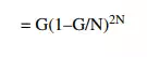
The core assumption of this model is that that a large number N of hosts are transmitting, each at a relatively low rate of s packets/slot. Denote by G the average number of transmission attempts per slot; we then have G = Ns. We will derive an expression for S, the average rate of successful transmissions per slot, in terms of G.

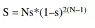
If two packets overlap during transmissions, both are lost. Thus, a successful transmission requires everyone else quiet for an interval of 2T: if a sender succeeds in the interval from t to t+T, then no other node can have tried to begin transmission in the interval t–T to t+T. The probability of one station transmitting during an interval of time T is G = Ns; the probability of the remaining N–1 stations all quiet for an interval of 2T is (1–s)2(N–1). The probability of a successful transmission is thus