Dynamic Range Enhancement for Automated Ultrasonic Testing of Composites

Dynamic range of advanced ultrasonic systems

Aerospace composite materials and structures take many forms, from thin plates to complex 3D shapes. One of the challenges of inspecting the more complex structures while using ultrasonic systems is to maintain a good SNR in all portions of the part. This can be particularly problematic when inspecting structures presenting large thickness variations or different material composition.

Panels bonded to honeycomb cores are good examples of such challenging structures. Ultrasonic testing of these types of materials is typically performed by transmitting ultrasounds through the thickness of the material (through-transmission), anomalies being identified by any loss of transmitted signal.

When adjusting the sensitivity of the ultrasonic instrument, the amplitude of the signals transmitted through the material must be kept below saturation in order to have reference levels for amplitude drop sizing. The attenuation of ultrasounds is typically very small for a skin-to-skin bond (no honeycomb). Sensitivity (gain) must therefore be kept low when we need to detect any indications in these structures. On the other hand, the attenuation is naturally high in honeycomb structures. Inspecting a structure presenting portions with and without honeycomb therefore presents a challenge to set the instrument sensitivity. Adjusting the gain on the skin material can result in a low contrast and poor SNR in the honeycomb structure. A high dynamic range (ratio between the largest and smallest meaningful signal amplitude) is required to detect defects in both sections of the material from a single gain setting.

What dynamic range is needed?

The dynamic range required to inspect a given structure is a function of the variation of attenuation within the structure and the required SNR. For example, in order to inspect a structure presenting differences of attenuation of 30 dB and where defects must be detected with a SNR of 16 dB, we will then require a system to have a dynamic range of at least 46 dB. In practice, a dynamic range as high as 90dB is rarely necessary.

Logarithmic Amplifiers

Logarithmic amplifiers (Log amps) have been widely used to perform ultrasonic testing of composite structures. The logarithmic amplification increases the dynamic range by performing a non-linear amplification of the ultrasonic signal in order to output a signal that is linear on a logarithmic scale. In practice, this means that signals of low amplitude are amplified at a higher dB level than the highest amplitude in the acquired A-Scans. The output of the logarithmic amplifier is a modified A-Scan which ertical scale is proportional to dB instead of Volts, yet represented on a volt or %FSH scale. When used by automated ultrasonic testing systems, a logarithmic amplifier allows for the production of C-Scans that have a high contrast between transmitted signals and the noise baseline. On the other hand, contrasts are decreased between high and low amplitude transmitted signals. Finer details about the structures are therefore sacrificed to maintain a high SNR in all areas of the samples. This allows one to inspect the full sample all at once, without having to re-scan sections of the sample at different gains. Dynamic ranges of such apparatuses are specified around 90dB, however signals entering the logarithmic amplifier must be extremely low noise, otherwise the resulting dynamic range is highly compromised. For this reason, narrowband filters centered on the probe frequency are typically used to remove as much noise as possible from the ultrasonic signals before entering the log amp.

Decibel scaling of numerical data

Before the introduction of numerical data acquisition, decibel scaling of ultrasonic signals was only possible through the use of logarithmic amplifiers. With data acquisition, converting amplitude to a decibel scale is now an easy task. However, high resolution data acquisition must be performed in order to obtain a valid dB scale. C-Scans can therefore be produced on a dB scale as if a logarithmic amplifier was used. However, the vertical resolution of the numerical acquisition and the electronic noise would limit the dynamic range. As a result, contrast between high and “zero” amplitude signals is limited by the noise level. For example, if there is a noise baseline of 0.5%, the resulting amplitude referred to 100% will be -46dB on the decibel scale; this corresponds to the dynamic range of the system. In practice, similar ranges can be expected to be obtained using acquisition cards of 12 or 14 bits.

In the event that more dynamic range is required, our TecView™ UT software allows one to record ultrasonic data at different gains. A second C-Scan can therefore be acquired simultaneously at a higher gain; this allows an ease in increasing the effective dynamic range of the ultrasonic inspection. Two C-Scan images are generated by the process: one for the lower gain setting and a second for areas where attenuation is more important. Since defect analysis and sizing must be performed using a reference signal in the vicinity of the detected indication, the analysis of each zone is done on different C-Scan images.

Comparison between a logarithmic amplifier and numerical acquisition

The example below shows the results of an ultrasonic inspection performed using a 12 bit acquisition card compared to an inspection performed with a logarithmic amplifier. The inspected sample has a honeycomb structure bonded to composite plates. Teflon tapes serve to simulate disbonds in the sample. For both inspections, the A-Scan amplitude was set to 80% of the full screen height at the reference location. This implied reducing the energy of the emitted pulse until the output signal of the logarithmic amplifier was at 80% of the screen at the reference point.

The images below shows the C-Scan obtained without the logarithmic amplifier by maximizing the echo signal amplitude in the skin area. The dark blue area represents the honeycomb structure area; this image is a good example of the poor contrast that results from large attenuation difference within a single sample. Here, there is a difference of approximately 29 dB between the maximum response from the skin and the response from the honeycomb structure.

C-Scan of disbonds (linear amplitude scale)

The following images compare the C-Scan obtained using the logarithmic amplifier (left) with the C-Scan obtained by converting the above C-Scan on a decibel scale (right). It is obvious from these images that the decibel conversion replicates the effects of the logarithmic amplifier. The color (amplitude level) of the defects is the only visible difference between both images; the use of the logarithmic amplifier resulted in a better color contrast for the detected defects. However, the amplitude corresponding to each pixel of the C-Scan obtained with the log amp does not have any physical meaning unless it is converted to dB; the calibration curve of the logarithmic must be known for this purpose. Conventional defect sizing (e.g. –X dB drop sizing) can only be achieved on the C-Scan on the right.

C-Scan with log amp.

C-Scan with gain 1

The log amplifier used during the scan tests was experimentally calibrated creating a table a table of calibration data from key sample points. This table was applied to the obtained C-Scan in order to convert it to a meaningful C-Scans with dB scale.

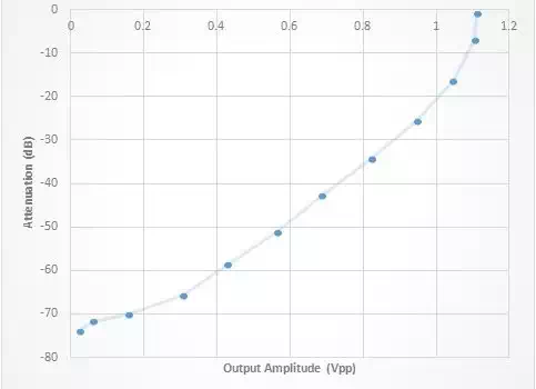
Calibration curve of the log amp; note the non-linearity of the response near 0dB and below -65 dB

Based on this calibration curve, the C-Scan obtained with the log amp has been converted to a dB scale and compared to the C-Scan obtained by numerical calculation of the dB scale.

C-Scan log amp in dB

C-Scan with gain 1

After rectification of the C-Scan on a real dB scale, it becomes apparent that the true dynamic range obtained with the log amp is not as high as it appeared to be. In this case, the true dynamic range obtained with the log amp is approximately 36 dB, while it is 44.8 dB on the regular C-Scan (produced from the linear A-Scans). The dB difference between the honeycomb core and the defect used for the example above is not as important for the scan done with the log amp (9.9 dB difference) as it is with the regular scan (12.4 dB difference).

It must be noted that the dynamic range obtained with the log amp could have been higher. Our results with the log amplifier are based on adjusting the reference signal at 80%; looking at the calibration curve of the log amp, we can see that setting the A-Scan at 80% (0.8Vpp) meant that the reference signal has already been attenuated by approximately 36 dB. However, if the reference signal had been saturated to 100% of the screen (1 Vpp) instead of 80%, the dynamic range of the log amplifier would have added 16dB bringing the overall increase to 52 dB; this is far from the specified 90dB amplification and is comparable to the dynamic range obtained with the 12 bit acquisition.

Enhanced dynamic range C-Scan acquisition

The dynamic range can be increased without using a log amp by using a two C-Scans acquired simultaneously but at different linear gains. Inspection tests were performed on the same sample where the second recorded C-Scan is 29 dB higher. The following results show the two recoded C-Scans. The image on the right shows the decibel scale representation of this second recorded C-Scan. The signal contrast in the reference area was increased to 35.9 dB in the second C-Scan (recorded with an additional 29dB). The dynamic range therefore was increased from approximately 44.8 dB to 68.3dB for the combined C-Scans.

C-Scan with gain 1

C-Scan gain 2 (additional 29 dB)

The dynamic range resulting from the dual gain approach is therefore well adapted to the part being inspected. In addition, it allows us to perform quantitative dB drop sizing without requiring any special calibration curves. With this approach, the recorded signals for the C-Scans are linear and the benefits of the logarithmic amplifier are reproduced without its negative aspects: – difficulty to interpret the amplitude information -the high sensitivity to electronic noise -the necessity to limit the bandwidth of the logarithmic amplifier around the probe frequency.