Automated Ultrasonic Scanners: Impact of Axes Misalignment

Ultrasonic testing using immersion or squirter systems require appropriate metrological calibration and alignment in order to provide excellent system performances including repeatability and defect detectability. In addition, the required performances of the automated UT system are related to the targeted inspection application. Simple applications where large defects are sought may only require basic system alignment and calibration. However, for advanced 2D & 3D ultrasonic testing and scanning, tighter system alignment needs to be achieved, with values which would guarantee optimal stability of the UT system, therefore allowing the probe to be perfectly perpendicular to the tested part.

Case study

To evaluate the targeted system alignment, tests were performed on woven composite samples where the variations of UT results (C-Scans) as a function of controlled mechanical deviations were evaluated. A 10-axis automated gantry/squirter scanning system was used to perform the measurements. The evaluated sample is a 12mm thick flat plate composite panel. Defects were simulated using 9 square Teflon® inserts with 0.25”, 0.5” and 1” dimension.

Scan setup and axes directions for the flat plate

Scan Results

A reference scan was performed on the flat woven composite sample before each misalignment test sequence. Prior to this inspection, squirters were carefully aligned in order to provide the most effective signal transmission through the sample. A scan was performed and then used as a comparative reference for all other scans performed following a controlled axes misalignment.
All C-scans were made at a 1 mm resolution and a water path of 110 mm using a 6 mm water jet. Data was acquired at a 25 MHz sample rate and with a precision of 14 bits.

C-Scan color palette of defects

For each scan, the sensitivity was adjusted until the baseline amplitude was approximately 80%, i.e the gain was adjusted between each misalignment in order to readjust the reference amplitude to ~80%.

Linear misalignment: (Y & Z direction)

In terms of the Z & Y directions, a linear misalignment of emitter probe relative to receiving probe along the Z-axis was first tested then followed by test in the Y-axis. Scans were made with probe misalignment increments of 1 to 2mm up to a maximum ±12mm relative to the reference scan.

C-Scans from different misalignment in Z (misalignment in mm is indicated above each C-Scan image)

Following misalignment in Y and Z, a comparison between the results obtained was done in order to confirm the independence of the results as a function of direction. A good correlation can be observed between the results obtained in both directions, confirming that there is no directivity effect for linear probe misalignment on the sample. The data analysis was done by measuring the difference between the minimum amplitude of each indication and the amplitude value found at the histogram peak for each C-Scan image (roughly corresponding to the average response of the background). As expected, the variation is symmetrical for both positive and negative misalignment.

Comparison of the difference between the minimum signal amplitude of each defect and the histogram peak of the corresponding C-Scan image as a function of combined misalignment in Y (solid lines) and a misalignment in Z (dotted lines)

Defect sizing was also evaluated as a function of probe misalignment. Again, no difference is observed between a misalignment in Y or Z and constant defect sizing was observed for a fairly wide misalignment. Defects of 0.5” and 1” are properly sized for misalignment up to +/- 10 mm, while only the 0.25mm is not properly sized above +/- 5 mm.

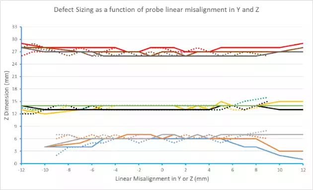
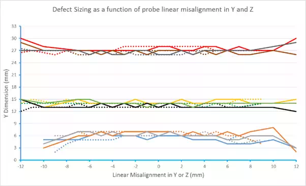
Comparison of the dimension of each defect obtained at 6dB below the histogram peak amplitude as a function of independent misalignments in Y (solid lines) and Z (dotted lines). a) Dimension along the Y axis; b) Dimension along the Z axis

This study was also extended to evaluate the angular misalignment of the probe and combination of both linear and angular misalignment. The results showed that for this type of composite material, the outcome on defect sizing and signal-to-noise ratio are dependent on the equivalent linear misalignment on the material surface rather than the angular offset itself.

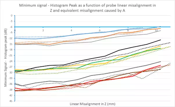
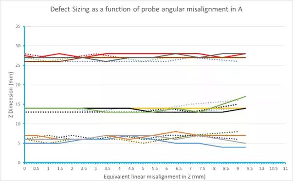
a) Comparison of the difference between the minimum signal amplitude of each defect and the histogram peak of the corresponding C-Scan image as a function of misalignment in Z (dotted lines) and the equivalent misalignment caused by an angular offset (solid lines). b) Comparison of the Z dimension of the defects under the same configuration.

Conclusions

This case study has provided interesting insights about effects of mechanical system alignment and its impact on defect detection in a woven composite materials. The conclusion of this case study is that the interaction of the ultrasound with the material that is inspected by a scanner has an impact on the required mechanical tolerances.