Oceanic Internal Waves
Introduction
Internal waves are waves in the interior of the ocean. They exist when the water body consists of layers of different density. This difference in water density is mostly due to a difference in water temperature, but can also be due to a difference in salinity. Often the density structure of the ocean can be approximated by two layers. The interface between layers of different densities is called pycnoline. When the density difference is due to temperature it is called thermocline, and when it is due to salinity it is called halocline.
Like the well-known ocean surface waves, which are waves at the interface of two media of different density, i. e., of water and air, the internal waves are waves at the interface between two water layers of different density. In both cases the restoring force is gravity, which is the reason why both waves sometimes are called gravity waves. These waves are generated when the interface is disturbed. In the case of surface waves, this disturbance can be caused by a stone thrown into the water or by wind blowing over the water surface. In the case of internal waves, this disturbance is usually caused by tidal flow pushing the layered water body over shallow underwater obstacles, e. g., over shallow sills or shallow ridges (Maxworthy, 1975, Helferich et al., 1984, Lamb, 1994).
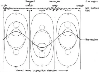
Internal waves in the ocean typically have wavelengths from hundreds of meters to tens of kilometers and periods from tens of minutes to several hours. Their amplitude (peak-to trough distance) often exceeds 50 m. Associated with internal waves are orbital motions of the water particles as depicted in Fig. 1 (the dashed circular lines). The radius of the circular motion of the water particles is largest at the pycnocline (or thermocline) depth and decreases downwards as well as upwards from this depth. To first order, the internal waves do not give rise to an elevation of the sea surface as the familiar surface waves do, but they do give rise to a variable (horizontal) surface current. The current velocity at the sea surface varies in magnitude and direction giving rise to convergent and divergent flow regimes at the sea surface as depicted in Fig. 1. The variable surface current interacts with the surface waves and modulates the sea surface roughness (Hughes, 1978, Alpers, 1985). This interaction is the reason why oceanic internal waves become visible on radar images of the sea surface and, in some cases, also on images acquired in the visible ultraviolet or infrared wavelength band (see, e. g., Apel et al., 1975).
Due to the hydrodynamic interaction of the variable surface current with the surface waves, the amplitude of the Bragg waves is increased in convergent flow regions and is decreased in divergent flow regions. As a consequence, the radar signatures of oceanic internal waves consist of alternating bright and dark bands on a uniform background.
But there exist also other radar signatures of internal waves: Sometimes they consist only of bright lines or only of dark bands. When the wind speed is below threshold for Bragg wave generation, only bright bands are encountered and when surface slicks are present, only dark lines are seen (da Silva et al., 1998). However, radar imaging theories capable of explaining these exceptional radar signatures of internal waves quantitatively still do not exist.
The tidally generated internal waves are usually highly nonlinear and occur often in wave packets. The distance between the waves in a wave packet and also the amplitude decrease from the front to the back. The amplitude of large internal waves can exceed 50 m in some cases. Theoretically, these highly nonlinear waves are often described in terms of internal solitons. Thus a wave packet consists of several solitons. Since soliton theory was developed by Korteweg and De Vries (1895), hundreds of papers have been published dealing with this subject. Soliton theories applicable to the description of the generation and propagation of internal solitary waves predict that, if the depth of the upper water layer is much smaller than the depth of the lower layer, then the internal solitary wave must be a "wave of depression". This means that this soliton is associated with a depression of the pycnocline as depicted schematically in Fig. 2 and as measured in the ocean (see Fig. 3). The leading edge of a soliton of depression is always associated with a convergent surface current region and the trailing edge with a divergent region. At the front of the soliton the amplitude of the Bragg waves is increased, while at the rear it is decreased. According to Bragg scattering theory, the normalized radar cross section (NRCS) is proportional to the amplitude squared of the Bragg wave (Valenzuela, 1978). This is the reason why on SAR images the front section of a soliton of depression is bright, and the rear section dark (Alpers, 1985). As mentioned before, the radar signatures of internal solitary waves may deviate from this scheme when surface slicks are present or the wind speed is low.
Oceanic internal solitary waves have been observed in many parts of the world's ocean. A very comprehensive list of publications on observation of large internal waves has been compiled by M. Miyata of the University of Hawaii.
Fig. 1: Schematic plot of processes associated with the passage of a linear oceanic internal wave. Deformation of the thermocline (heavy solid line), orbital motions of the water particles (dashed lines), streamlines of the velocity field (light solid lines), surface current velocity vectors (arrows in the upper part of the image), and variation of the amplitude of the Bragg waves (wavy line at the top).
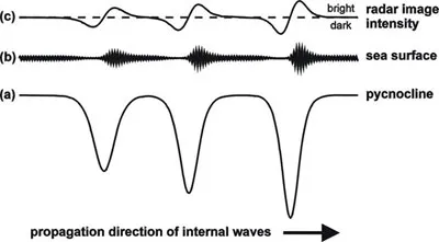
Fig. 2: Shape of the pynocline (a), sea surface roughness pattern (b), and SAR image intensity (c) associated with an internal solitary wave packet consisting of solitons of depression of decreasing amplitude.
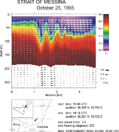
Fig. 3: Density and current distributions measured in the Mediterranean Sea north of the Strait of Messina during the passage of a northward propagating packet of internal solitary waves. The density distribution was measured by a CTD (conductivity temperature, depth) chain (Sellschopp, 1997) and the current distribution by an acoustic Doppler current profiler from the research ship "Alliance" (Figure provided by P. Brandt and A. Rubino, Institute of Oceanography, University of Hamburg).