Eigenvalues and Eigenvectors

Introduction

This page is a brief introduction to eigenvalue/eigenvector problems (don't worry if you haven't heard of the latter).  Before reading this you should feel comfortable with basic matrix operations.  If you are confident in your ability with this material, feel free to skip it.

Note that there is no description of how the operations are done -- it is assumed that you are using a calculator that can handle matrices, or a program like MatLab.  Also, this page typically only deals with the most general cases, there are likely to be special cases (for example, non-unique eigenvalues) that aren't covered at all.

Eigenvalues and Eigenvectors

Many problems present themselves in terms of an eigenvalue problem:

A·v=λ·v

In this equation A is an n-by-n matrix, v is a non-zero n-by-1 vector and λ is a scalar (which may be either real or complex).  Any value of λ for which this equation has a solution is known as an eigenvalue of the matrix A.  It is sometimes also called the characteristic value.  The vector, v, which corresponds to this value is called an eigenvector.  The eigenvalue problem can be rewritten as 

A·v-λ·v=0
A·v-λ·I·v=0
(A-λ·I)·v=0

If v is non-zero, this equation will only have a solution if 

|A-λ·I|=0

This equation is called the characteristic equation of A, and is an n^th order polynomial in λ with n roots.  These roots are called the eigenvalues of A.  We will only deal with the case of n distinct roots, though they may be repeated.  For each eigenvalue there will be an eigenvector for which the eigenvalue equation is true.  This is most easily demonstrated by example

Example: Find Eigenvalues and Eigenvectors of a 2x2 Matrix

If

then the characteristic equation is 

and the two eigenvalues are

λ₁=-1, λ₂=-2

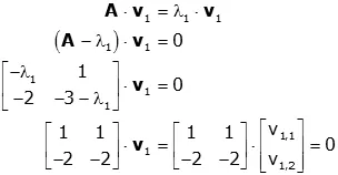
All that's left is to find the two eigenvectors.  Let's find the eigenvector, v₁, associated with the eigenvalue, λ₁=-1, first.

so clearly from the top row of the equations we get

Note that if we took the second row we would get

In either case we find that the first eigenvector is any 2 element column vector in which the two elements have equal magnitude and opposite sign.

where k₁ is an arbitrary constant.  Note that we didn't have to use +1 and -1, we could have used any two quantities of equal magnitude and opposite sign.

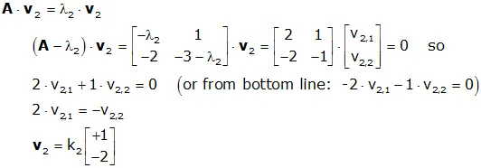
Going through the same procedure for the second eigenvalue:

 Again, the choice of +1 and -2 for the eigenvector was arbitrary; only their ratio is important.  This is demonstrated in the MatLab code below.

Using MatLab

>> A=[0 1;-2 -3]

A =

  0   1

 -2  -3

>> [v,d]=eig(A)

v =

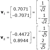
  0.7071  -0.4472

 -0.7071   0.8944

d =

 -1   0

  0  -2

The eigenvalues are the diagonal of the "d" matrix

 The eigenvectors are the columns of the "v" matrix. 

Note that MatLab chose different values for the eigenvectors than the ones we chose.  However, the ratio of v_1,1 to v_1,2 and the ratio of v_2,1 to v_2,2 are the same as our solution; the chosen eigenvectors of a system are not unique, but the ratio of their elements is.  (MatLab chooses the values such that the sum of the squares of the elements of each eigenvector equals unity).