Legendre polynomials
The Legendre polynomials, sometimes called Legendre functions of the first kind, Legendre coefficients, or zonal harmonics (Whittaker and Watson 1990, p. 302), are solutions to the Legendre differential equation. If ![]() is an integer, they are polynomials. The Legendre polynomials
is an integer, they are polynomials. The Legendre polynomials ![]() are illustrated above for
are illustrated above for  and
and ![]() , 2, ..., 5. They are implemented in the Wolfram Language as LegendreP[n, x].
, 2, ..., 5. They are implemented in the Wolfram Language as LegendreP[n, x].
The associated Legendre polynomials ![]() and
and ![]() are solutions to the associated Legendre differential equation, where
are solutions to the associated Legendre differential equation, where ![]() is a positive integer and
is a positive integer and ![]() , ...,
, ..., ![]() .
.
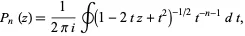
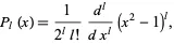
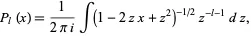
The Legendre polynomial ![]() can be defined by the contour integral
can be defined by the contour integral
| (1) |
where the contour encloses the origin and is traversed in a counterclockwise direction (Arfken 1985, p. 416).
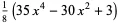
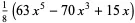
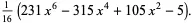
The first few Legendre polynomials are
|
|
| (2) |
|
|
| (3) |
|
|
| (4) |
|
|
| (5) |
|
|
| (6) |
|
|
| (7) |
|
|
| (8) |
When ordered from smallest to largest powers and with the denominators factored out, the triangle of nonzero coefficients is 1, 1
![]() , 3,
, 3, ![]() , 5, 3,
, 5, 3, ![]() , ... (OEIS A008316). The leading denominators are 1, 1, 2, 2, 8, 8, 16, 16, 128, 128, 256, 256, ... (OEIS A060818).
, ... (OEIS A008316). The leading denominators are 1, 1, 2, 2, 8, 8, 16, 16, 128, 128, 256, 256, ... (OEIS A060818).
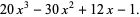
The first few powers in terms of Legendre polynomials are
|
|
| (9) |
|
|
| (10) |
|
|
| (11) |
|
|
| (12) |
|
|
| (13) |
|
|
| (14) |
(OEIS A008317 and A001790). A closed form for these is given by
| (15) |
(R. Schmied, pers. comm., Feb. 27, 2005). For Legendre polynomials and powers up to exponent 12, see Abramowitz and Stegun (1972, p. 798).
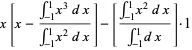
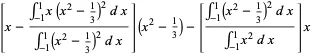
The Legendre polynomials can also be generated using Gram-Schmidt orthonormalization in the open interval ![]() with the weighting function 1.
with the weighting function 1.
|
|
| (16) |
|
|
| (17) |
|
|
| (18) |
|
|
| (19) |
|
|
| (20) |
|
|
| (21) |
|
|
| (22) |
Normalizing so that  gives the expected Legendre polynomials.
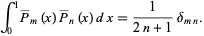
The "shifted" Legendre polynomials are a set of functions analogous to the Legendre polynomials, but defined on the interval (0, 1). They obey the orthogonality relationship
| (23) |
The first few are
|
|
| (24) |
|
|
| (25) |
|
|
| (26) |
|
|
| (27) |
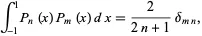
The Legendre polynomials are
orthogonal over ![]() with weighting function 1 and satisfy
with weighting function 1 and satisfy
| (28) |
where ![]() is the Kronecker delta.
is the Kronecker delta.
The Legendre polynomials are a special case of the Gegenbauer polynomials with ![]() , a special case of the Jacobi polynomials
, a special case of the Jacobi polynomials ![]() with
with  , and can be written as a hypergeometric function using Murphy's formula
| (29) |
(Bailey 1933; 1935, p. 101; Koekoek and Swarttouw 1998).
The Rodrigues representation provides the formula
| (30) |
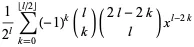
which yields upon expansion
|
|
| (31) |
|
|
| (32) |
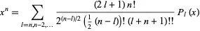
where ![]() is the floor function. Additional sum formulas include
is the floor function. Additional sum formulas include
|
|
| (33) |
|
|
| (34) |
(Koepf 1998, p. 1). In terms of hypergeometric functions, these can be written
|
|
| (35) |
|
|
| (36) |
|
|
| (37) |
(Koepf 1998, p. 3).
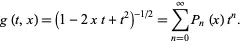
A generating function for ![]() is given by
is given by
| (38) |
Take ![]() ,
,
| (39) |
Multiply (39) by ![]() ,
,
| (40) |
and add (38) and (40),
| (41) |
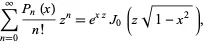
This expansion is useful in some physical problems, including expanding the Heyney-Greenstein phase function and computing the charge distribution on a sphere. Another generating function is given by
| (42) |
where ![]() is a zeroth order Bessel function of the first kind (Koepf 1998, p. 2).
is a zeroth order Bessel function of the first kind (Koepf 1998, p. 2).
The Legendre polynomials satisfy the recurrence relation
| (43) |
(Koepf 1998, p. 2). In addition,
| (44) |
(correcting Hildebrand 1956, p. 324).
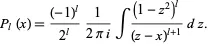
A complex generating function is
| (45) |
and the Schläfli integral is
| (46) |
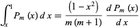
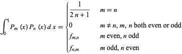
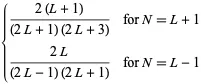
Integrals over the interval ![]() include the general formula
include the general formula
| (47) |
for ![]() (Byerly 1959, p. 172), from which the special case
(Byerly 1959, p. 172), from which the special case
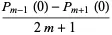
|
|
| (48) |
|
|
| (49) |
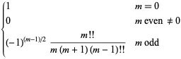
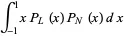
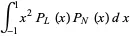
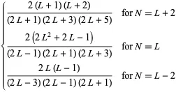
follows (OEIS A002596 and A046161; Byerly 1959, p. 172). For the integral over a product of Legendre functions,
| (50) |
for ![]() (Byerly 1959, p. 172), which gives the special case
(Byerly 1959, p. 172), which gives the special case
| (51) |
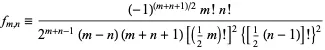
where
| (52) |
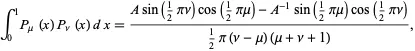
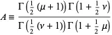
(OEIS A078297 and A078298; Byerly 1959, p. 172). The latter is a special case of
| (53) |
where
| (54) |
and ![]() is a gamma function (Gradshteyn and Ryzhik 2000, p. 762, eqn. 7.113.1)
is a gamma function (Gradshteyn and Ryzhik 2000, p. 762, eqn. 7.113.1)
Integrals over ![]() with weighting functions
with weighting functions ![]() and
and ![]() are given by
are given by
|
|
| (55) |
|
|
| (56) |
(Arfken 1985, p. 700).
The Laplace transform is given by
| (57) |
where ![]() is a modified Bessel function of the first kind.
is a modified Bessel function of the first kind.
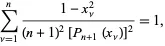
A sum identity is given by
| (58) |
where ![]() is the
is the ![]() th root of
th root of ![]() (Szegö 1975, p. 348). A similar identity is
(Szegö 1975, p. 348). A similar identity is
| (59) |