Correlation and regression

The word correlation is used in everyday life to denote some form of association. We might say that we have noticed a correlation between foggy days and attacks of wheeziness. However, in statistical terms we use correlation to denote association between two quantitative variables. We also assume that the association is linear, that one variable increases or decreases a fixed amount for a unit increase or decrease in the other. The other technique that is often used in these circumstances is regression, which involves estimating the best straight line to summarise the association.

Correlation coefficient

The degree of association is measured by a correlation coefficient, denoted by r. It is sometimes called Pearson's correlation coefficient after its originator and is a measure of linear association. If a curved line is needed to express the relationship, other and more complicated measures of the correlation must be used.

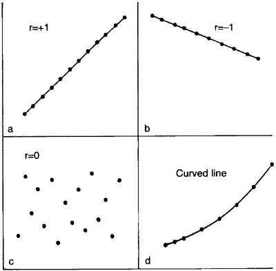
The correlation coefficient is measured on a scale that varies from + 1 through 0 to - 1. Complete correlation between two variables is expressed by either + 1 or -1. When one variable increases as the other increases the correlation is positive; when one decreases as the other increases it is negative. Complete absence of correlation is represented by 0. Figure 11.1 gives some graphical representations of correlation.

Figure 11.1 Correlation illustrated.

Looking at data: scatter diagrams

When an investigator has collected two series of observations and wishes to see whether there is a relationship between them, he or she should first construct a scatter diagram. The vertical scale represents one set of measurements and the horizontal scale the other. If one set of observations consists of experimental results and the other consists of a time scale or observed classification of some kind, it is usual to put the experimental results on the vertical axis. These represent what is called the "dependent variable". The "independent variable", such as time or height or some other observed classification, is measured along the horizontal axis, or baseline.

The words "independent" and "dependent" could puzzle the beginner because it is sometimes not clear what is dependent on what. This confusion is a triumph of common sense over misleading terminology, because often each variable is dependent on some third variable, which may or may not be mentioned. It is reasonable, for instance, to think of the height of children as dependent on age rather than the converse but consider a positive correlation between mean tar yield and nicotine yield of certain brands of cigarette.' The nicotine liberated is unlikely to have its origin in the tar: both vary in parallel with some other factor or factors in the composition of the cigarettes. The yield of the one does not seem to be "dependent" on the other in the sense that, on average, the height of a child depends on his age. In such cases it often does not matter which scale is put on which axis of the scatter diagram. However, if the intention is to make inferences about one variable from the other, the observations from which the inferences are to be made are usually put on the baseline. As a further example, a plot of monthly deaths from heart disease against monthly sales of ice cream would show a negative association. However, it is hardly likely that eating ice cream protects from heart disease! It is simply that the mortality rate from heart disease is inversely related - and ice cream consumption positively related - to a third factor, namely environmental temperature.

Calculation of the correlation coefficient

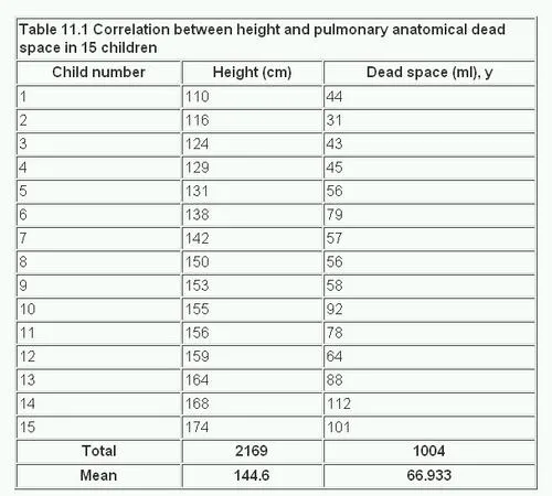
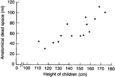
A paediatric registrar has measured the pulmonary anatomical dead space (in ml) and height (in cm) of 15 children. The data are given in table 11.1 and the scatter diagram shown in figure 11.2 Each dot represents one child, and it is placed at the point corresponding to the measurement of the height (horizontal axis) and the dead space (vertical axis). The registrar now inspects the pattern to see whether it seems likely that the area covered by the dots centres on a straight line or whether a curved line is needed. In this case the paediatrician decides that a straight line can adequately describe the general trend of the dots. His next step will therefore be to calculate the correlation coefficient.

When making the scatter diagram (figure 11.2 ) to show the heights and pulmonary anatomical dead spaces in the 15 children, the paediatrician set out figures as in columns (1), (2), and (3) of table 11.1 . It is helpful to arrange the observations in serial order of the independent variable when one of the two variables is clearly identifiable as independent. The corresponding figures for the dependent variable can then be examined in relation to the increasing series for the independent variable. In this way we get the same picture, but in numerical form, as appears in the scatter diagram.

Figure 11.2 Scatter diagram of relation in 15 children between height and pulmonary anatomical dead space.

The calculation of the correlation coefficient is as follows, with x representing the values of the independent variable (in this case height) and y representing the values of the dependent variable (in this case anatomical dead space). The formula to be used is:

which can be shown to be equal to:

Calculator procedure

Find the mean and standard deviation of x, as described in 

Find the mean and standard deviation of y: 

Subtract 1 from n and multiply by SD(x) and SD(y), (n - 1)SD(x)SD(y)

This gives us the denominator of the formula. (Remember to exit from "Stat" mode.)

For the numerator multiply each value of x by the corresponding value of y, add these values together and store them.

110 x 44 = Min

116 x 31 = M+

etc.

This stores  in memory. Subtract 

MR - 15 x 144.6 x 66.93 (5426.6)

Finally divide the numerator by the denominator.

r = 5426.6/6412.0609 = 0.846.

The correlation coefficient of 0.846 indicates a strong positive correlation between size of pulmonary anatomical dead space and height of child. But in interpreting correlation it is important to remember that correlation is not causation. There may or may not be a causative connection between the two correlated variables. Moreover, if there is a connection it may be indirect.

A part of the variation in one of the variables (as measured by its variance) can be thought of as being due to its relationship with the other variable and another part as due to undetermined (often "random") causes. The part due to the dependence of one variable on the other is measured by Rho . For these data Rho= 0.716 so we can say that 72% of the variation between children in size of the anatomical dead space is accounted for by the height of the child. If we wish to label the strength of the association, for absolute values of r, 0-0.19 is regarded as very weak, 0.2-0.39 as weak, 0.40-0.59 as moderate, 0.6-0.79 as strong and 0.8-1 as very strong correlation, but these are rather arbitrary limits, and the context of the results should be considered.