First-Order Homogeneous Ode

WHAT IS A FIRST-ORDER HOMOGENEOUS ODE?

Now any differential equation with $\cfrac{dy}{dx}$ is a first-order ODE. This type of equation does not have any higher-order derivative.

Next is ‘homogeneous.’

Now any first-order ODE is homogeneous if the total degree for each term is the same.

For example, 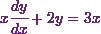$x\cfrac{dy}{dx} + 2y = 3x$ is a first-order homogeneous ODE. This is because each term has a degree 1.

Again, 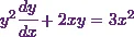$y^2\cfrac{dy}{dx} + 2xy = 3x^2$ is also a first-order homogeneous ODE. This is because each term has a total degree as 2.

But 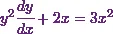$y^2\cfrac{dy}{dx} + 2x = 3x^2$ is not a homogeneous ODE. This is because each term does not have the same degree.

HOW CAN I SOLVE A FIRST-ORDER HOMOGENEOUS ODE?

Now there is a standard method to solve any first-order homogeneous ODE.

That is,

Choose y = vx .

Replace and $\cfrac{dy}{dx}$ with and $\cfrac{dv}{dx}$ respectively.

Solve the equation.

Bring back .

Next, I will solve an example on the first-order homogeneous ODE.

EXAMPLE

According to Stroud and Booth (2013)* “Find the general solution of 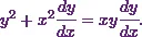$y^2+ x^2\cfrac{dy}{dx} = xy \cfrac{dy}{dx}.$ ”

SOLUTION

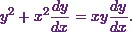
Here the given ordinary differential equation (ODE) is:

$y^2+ x^2\cfrac{dy}{dx} = xy \cfrac{dy}{dx}.$

This equation has only $\cfrac{dy}{dx}$ and no $\cfrac{d^2y}{dx^2}.$ Hence this is a first-order ODE.

Now, in this equation, each term has a total degree of .

For example, y^2 has a degree .

Similarly, x^2 has the same degree of .

But the term has the total degree as . This is because has a degree of and also has a degree of .

So together it’s (1+1) = 2 .

Thus I can say that this is a homogeneous equation.

Now I’ll solve this equation using the same method as I’ve described above.

STEP 1

First of all, I’ll give this equation a number, say,

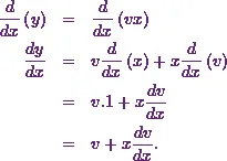
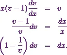
(1) $\begin{equation*} y^2+ x^2\frac{dy}{dx} = xy \frac{dy}{dx}. \end{equation*}$

Now I choose y = vx .

Therefore, I’ll differentiate with respect to . For that, I’ll use the product rule of differentiation.

Thus it will be

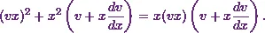
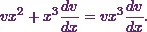
$\begin{eqnarray*} \frac{d}{dx}\left(y\right )&=& \frac{d}{dx}\left(vx\right)\\ \frac{dy}{dx} &=& v \frac{d}{dx}\left(x\right)+ x\frac{d}{dx}\left(v\right)\\ &=& v . 1 + x\frac{dv}{dx}\\&=& v + x\frac{dv}{dx}. \end{eqnarray*}$

Now I’ll substitute y = vx and $\cfrac{dy}{dx} = v + x\cfrac{dv}{dx}$ in equation (1).

Thus it will be

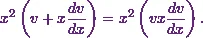
$\begin{equation*} (vx)^2+ x^2\left( v + x\frac{dv}{dx}\right) = x(vx) \left( v + x\frac{dv}{dx}\right). \end{equation*}$

Now I’ll simplify it to get

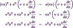
$\begin{eqnarray*} (vx)^2+ x^2\left( v + x\frac{dv}{dx}\right) &=& x(vx) \left( v + x\frac{dv}{dx}\right)\\ v^2x^2+ vx^2 + x^3\frac{dv}{dx} &=& vx^2 \left( v + x\frac{dv}{dx}\right)\\ v^2x^2+ vx^2 + x^3\frac{dv}{dx} &=& v^2x^2 + vx^3\frac{dv}{dx}. \end{eqnarray*}$

Next I’ll cancel v^2x^2 to get

$\begin{equation*} vx^2 + x^3\frac{dv}{dx} = vx^3\frac{dv}{dx}. \end{equation*}$

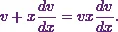
Now I can see that each term also has x^2 as a common term.

So I’ll take that out like

$\begin{equation*} x^2\left(v + x\frac{dv}{dx}\right) =x^2\left(vx\frac{dv}{dx}\right). \end{equation*}$

Since $x^2 \neq 0,$ I can cancel that from both sides of the equation.

Thus it becomes

(2) $\begin{equation*} v + x\frac{dv}{dx} = vx\frac{dv}{dx}. \end{equation**}$

It’s not possible to simplify it any more.

So now my job is to solve it.

STEP 2

First of all, I’ll take the $\cfrac{dv}{dx}$ term on one side.

So equation (2) will be

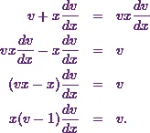
$\begin{eqnarray*} v + x\frac{dv}{dx} &=& vx\frac{dv}{dx}\\ vx\frac{dv}{dx} - x\frac{dv}{dx} &=& v\\ (vx - x)\frac{dv}{dx} &=& v\\ x(v - 1)\frac{dv}{dx} &=& v. \end{eqnarray*}$

Now it’s very clear that I can separate and variables to solve the equation.

In other words, I’ll use ‘separation of variables’ method to solve this equation.

Therefore the equation will be

$\begin{eqnarray*} x(v - 1)\frac{dv}{dx} &=& v\\ \frac{v-1}{v}dv &=& \frac{dx}{x}\\\left(1 - \frac{1}{v}\right) dv &=& dx. \end{eqnarray*}$

Now I’ll integrate both sides of the equation to get .

Thus it will be

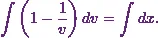
$\begin{equation*} \int \left(1 - \frac{1}{v}\right) dv = \int dx. \end{equation*}$

So this gives

$v - \ln v &=& \ln x + \ln C.$

Here is the integration constant.

As a next step, I’ll bring back in the solution.

STEP 3

Next, I’ll replace with $\cfrac{y}{x}$ .

So it will be

$\frac{y}{x}- \ln \frac{y}{x} = \ln x + \ln C.$

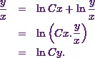
Now I’ll bring logarithmic expressions on one-side.

Therefore it becomes

$\frac{y}{x} = \ln x + \ln C + \ln \frac{y}{x}.$

Next, I’ll work on the logarithmic functions of this solution.

As I already know $\ln ab = \ln a + \ln b$ , I can say $\ln x + \ln C = \ln Cx$ .

So the equation will become

$\begin{eqnarray*} \frac{y}{x} &=& \ln Cx + \ln \frac{y}{x}\\ &=& \ln \left(Cx. \frac{y}{x}\right)\\ &=& \ln Cy. \end{eqnarray*}$

Next I’ll take anti-logarithm on both sides.

Thus it will be

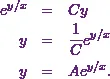
$\begin{eqnarray*} e^{y/x} &=& Cy\\ y &=& \frac{1}{C}e^{y/x}\\ y &=& A e^{y/x}. \end{eqnarray*}$

Here $A = \cfrac{1}{C}.$

Hence I can conclude that the general solution of the equation is $y = A e^{y/x}.$

This is the answer to this example.