Bootstrap technique

Bootstrapping is a statistical procedure that resamples a single dataset to create many simulated samples. This process allows you to calculate standard errors, construct confidence intervals, and perform hypothesis testing for numerous types of sample statistics. Bootstrap methods are alternative approaches to traditional hypothesis testing and are notable for being easier to understand and valid for more conditions.

In this blog post, I explain bootstrapping basics, compare bootstrapping to conventional statistical methods, and explain when it can be the better method. Additionally, I’ll work through an example using real data to create bootstrapped confidence intervals.

Bootstrapping and Traditional Hypothesis Testing Are Inferential Statistical Procedures

Both bootstrapping and traditional methods use samples to draw inferences about populations. To accomplish this goal, these procedures treat the single sample that a study obtains as only one of many random samples that the study could have collected.

From a single sample, you can calculate a variety of sample statistics, such as the mean, median, and standard deviation—but we’ll focus on the mean here.

Now, suppose an analyst repeats their study many times. In this situation, the mean will vary from sample to sample and form a distribution of sample means. Statisticians refer to this type of distribution as a sampling distribution. Sampling distributions are crucial because they place the value of your sample statistic into the broader context of many other possible values.

While performing a study many times is infeasible, both methods can estimate sampling distributions. Using the larger context that sampling distributions provide, these procedures can construct confidence intervals and perform hypothesis testing.

Related posts: Differences between Descriptive and Inferential Statistics

Differences between Bootstrapping and Traditional Hypothesis Testing

A primary difference between bootstrapping and traditional statistics is how they estimate sampling distributions.

Traditional hypothesis testing procedures require equations that estimate sampling distributions using the properties of the sample data, the experimental design, and a test statistic. To obtain valid results, you’ll need to use the proper test statistic and satisfy the assumptions. I describe this process in more detail in other posts—links below.

The bootstrap method uses a very different approach to estimate sampling distributions. This method takes the sample data that a study obtains, and then resamples it over and over to create many simulated samples. Each of these simulated samples has its own properties, such as the mean. When you graph the distribution of these means on a histogram, you can observe the sampling distribution of the mean. You don’t need to worry about test statistics, formulas, and assumptions.

The bootstrap procedure uses these sampling distributions as the foundation for confidence intervals and hypothesis testing. Let’s take a look at how this resampling process works.

Related posts: How t-Tests Work and How the F-test Works in ANOVA

How Bootstrapping Resamples Your Data to Create Simulated Datasets

Bootstrapping resamples the original dataset with replacement many thousands of times to create simulated datasets. This process involves drawing random samples from the original dataset. Here’s how it works:

1. The bootstrap method has an equal probability of randomly drawing each original data point for inclusion in the resampled datasets.

2. The procedure can select a data point more than once for a resampled dataset. This property is the “with replacement” aspect of the process.

3. The procedure creates resampled datasets that are the same size as the original dataset.

The process ends with your simulated datasets having many different combinations of the values that exist in the original dataset. Each simulated dataset has its own set of sample statistics, such as the mean, median, and standard deviation. Bootstrapping procedures use the distribution of the sample statistics across the simulated samples as the sampling distribution.

Example of Bootstrap Samples

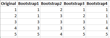
Let’s work through an easy case. Suppose a study collects five data points and creates four bootstrap samples, as shown below.

This simple example illustrates the properties of bootstrap samples. The resampled datasets are the same size as the original dataset and only contain values that exist in the original set. Furthermore, these values can appear more or less frequently in the resampled datasets than in the original dataset. Finally, the resampling process is random and could have created a different set of simulated datasets.

Of course, in a real study, you’d hope to have a larger sample size, and you’d create thousands of resampled datasets. Given the enormous number of resampled data sets, you’ll always use a computer to perform these analyses.