Lines and Cables

 The equivalent π-model of a transmission line section was derived in the lectures Electric Power Systems (Elektrische Energiesysteme), 227-0122-00L. The general distributed model is characterized by the series parameters

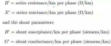
as depicted in Figure 2.1. The parameters above are specific for the line or cable configuration and are dependent on conductors and geometrical arrangements.

From the circuit in Figure 2.1 the telegraph equation is derived, and from this the lumped-circuit line model for symmetrical steady state conditions, Figure 2.2. This model is frequently referred to as the π-model, and it is characterized by the parameters

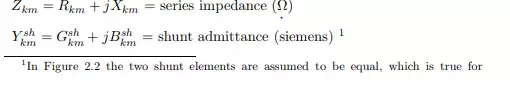
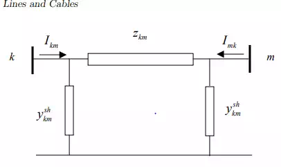
Lumped-circuit model (π-model) of a transmission line between nodes k and m.

Note. In the following most analysis will be made in the p.u. system. For impedances and admittances, capital letters indicate that the quantity is expressed in ohms or siemens, and lower case letters that they are expressed in p.u.

Note. In these lecture notes complex quantities are not explicitly marked as underlined. This means that instead of writing zkm we will write zkm when this quantity is complex. However, it should be clear from the context if a quantity is real or complex. Furthermore, we will not always use specific type settings for vectors. Quite often vectors will be denoted by bold face type setting, but not always. It should also be clear from the context if a quantity is a vector or a scalar.

When formulating the network equations the node admittance matrix will be used and the series admittance of the line model is needed

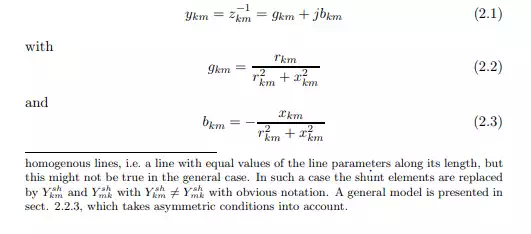
For actual transmission lines the series reactance xkm and the series resistance rkm are both positive, and consequently gkm is positive and bkm is negative. The shunt susceptance y sh km and the shunt conductance g sh km are both positive for real line sections. In many cases the value of g sh km is so small that it could be neglected.

 The complex currents Ikm and Imk in Figure 2.2 can be expressed as functions of the complex voltages at the branch terminal nodes k and m:

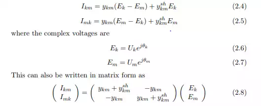
As seen the matrix on the right hand side of eq. (2.8) is symmetric and the diagonal elements are equal. This reflects that the lines and cables are symmetrical elements.

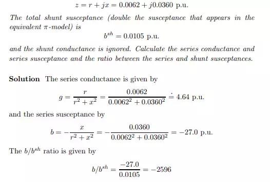
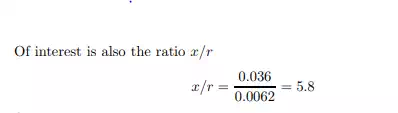
Example 2.1. The series impedance of a 138 kV transmission line section is