charge simulation method
Abstract
This paper deals with the calculation of the electric field strength in high voltage (HV) substations comprising complex geometrical structures. Generalized charge simulation method is proposed for improving the precision of the calculation of the electric field strength. The objective of this analysis is to examine the influence of towers, HV apparatus and fences on the spatial electric field distribution. For this purpose, a three-dimensional generalized model of HV substation has been developed, including phase conductors, bypass busbars, HV apparatus, fences and towers (denoted as Full model). The obtained results of the calculation of the electric field strength are compared with the Simplified model, which only includes phase conductors connected to HV network. Verification of the proposed Full model performed by comparing the calculated and in-field measured values of the electric field strength within HV substations and in their vicinity gives very promising results.
Introduction
One of the commonest sources of non-ionizing radiation that humans are exposed to is the industrial-frequency electromagnetic field. The effect of the electric field of an industrial frequency is especially important in the areas close to high voltage (HV) facilities. The electric field strength that occurs in the vicinity of HV facilities must not exceed the levels proposed by environmental and health regulations and standards [1,2]. The guidelines are 10 kV/m in occupational exposure and 5 kV/m in public exposure. For this reason, when drafting a project plan of a HV facility, it is very important to perform an estimation of the intensity of the electric field—inside the facility and in its immediate surrounding. The HV substation represents an especially complex case in this area, due to a great number of line conductors, towers, HV equipment and substation fences, following that all of them have an impact on the distribution of the electric field. There are various numerical methods for computing the electric field strength [3]: finite difference method (FDM), finite element method (FEM), boundary element method (BEM) and charge simulation method (CSM). Although being one of the simplest and oldest numerical methods, FDM suffers from relatively slow convergences. The FEMbased modelling of the partial differential equations is performed by discretizing the entire calculation domain into a grid of elements of finite size. The FEM can compute threedimensional (3D) electric field strength, but difficulties arise as the result of a large number of the system equations, which require more time for the computation and larger computer memory. The basic idea of BEM is to discretize the integral equation using boundary elements, where boundary surfaces are divided into a set of elements. The BEM is a convenient technique for the computation of the electric field strength close to the conductor surface, but is inadequate for computing a large number of linear conductors in the open space. In this case, the BEM requires more computer memory and computation time. The CSM has the advantage of being highly efficient in the calculation of the electric field strengthin the open space. Once the fictitious charges distribution for an observed configuration is determined, it is relatively easy to calculate the electric potential and the electric field strength at particular points using the superposition principle. In most of the papers presenting electric field calculation in the HV substation, only conductors of known potential are taken into consideration [4–6]. A more detailed model with influence of towers and HV apparatus based on CSM and BEM combination is given in [7]. In this paper, a generalized charge simulation model appropriate for the calculation of the electric field strength at both HV substations and in the vicinity is proposed. A detailed 3D model of HV substation (denoted as Full model), which includes conductors of known potential (phase conductors, main busbars, fences and towers), conductors at floating potential (bypass busbars)
Basic equations for the calculation of the electric field strength
The basic principle of CSM lies in replacing the surface charge of a conductor with a set of discrete fictitious charges, located inside the conductor. These fictitious charges applied in the presented model can be divided into the following types: 1. linear charge; 2. ring-shaped charge. Fictitious charges generate the electric field of similar intensity and direction as the original conductors in the observed zone. Fictitious linear charges are used for the modelling of the line conductors (phase conductors, main busbars, fences and towers, bypass busbars), as shown in Fig. 1a. Fictitious ringshaped charges are used for the modelling of the dielectric surface (HV apparatus), as shown in Fig. 1b.
The conductor with known potential
Although the type and position of fictitious charges inside the conductor are specified in advance, as shown in Fig. 1a, their values are unknown. In order to determine the value of nc, the fictitious charges at the conductor with known potential Vc, a certain number nCPc of contour points are selected. Although number of fictitious charges can be different from number of contour points, in this paper, a conventional application of the CSM is suggested when the condition nc = nCPc is satisfied. Contour points are placed at the conductor surface where the boundary conditions given by potentials of the contour points equal to Vc are satisfied. The potential of each contour
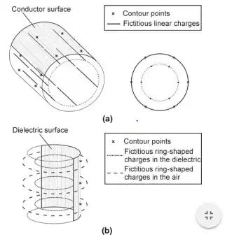
Fig. 1 Arrangement of fictitious charges and contour points point ic denoted by Vic is calculated by a superposition of the influences of all the existing fictitious charges Qc jc and must be equal to the potential of the conductor Vc according to [4,8]: nc jc=1 Pcic jc Qc jc = Vic and Vic = Vc, ic = 1, 2,... nc. (1) The potential coefficients Pcic jc are dependent on the type of the charge and the relative position r between the point ic at which the potential is calculated and the point jc, where the fictitious charge is placed. Assuming that all of the potentials are simple-periodic and of the same frequency, the system of equations (given in Eq. 1) can be presented in the complex form. The fictitious complex charges can be derived from the system of complex equations in the matrix form: [Pc] · Qc = Vc , with solution Qc = Pc 1 Vc , (2) where: [Pc] is the matrix of potential coefficients whose dimension is nc × nc, [Qc ] is the vector of unknown complex charges of the dimension nc