The Finite Element Method (FEM)

An Introduction to the Finite Element Method

The description of the laws of physics for space- and time-dependent problems are usually expressed in terms of partial differential equations (PDEs). For the vast majority of geometries and problems, these PDEs cannot be solved with analytical methods. Instead, an approximation of the equations can be constructed, typically based upon different types of discretizations. These discretization methods approximate the PDEs with numerical model equations, which can be solved using numerical methods. The solution to the numerical model equations are, in turn, an approximation of the real solution to the PDEs. The finite element method (FEM) is used to compute such approximations. Take, for example, a function u that may be the dependent variable in a PDE (i.e., temperature, electric potential, pressure, etc.) The function u can be approximated by a function u_h using linear combinations of basis functions according to the following expressions:

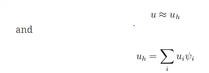
Here, ψ_i denotes the basis functions and u_i denotes the coefficients of the functions that approximate u with u_h. The figure below illustrates this principle for a 1D problem. u could, for instance, represent the temperature along the length (x) of a rod that is nonuniformly heated. Here, the linear basis functions have a value of 1 at their respective nodes and 0 at other nodes. In this case, there are seven elements along the portion of the x-axis, where the function u is defined (i.e., the length of the rod).

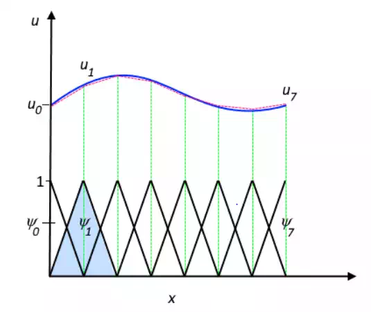
The function u (solid blue line) is approximated with u_h (dashed red line), which is a linear combination of linear basis functions (ψ_i is represented by the solid black lines). The coefficients are denoted by u₀ through u₇.

One of the benefits of using the finite element method is that it offers great freedom in the selection of discretization, both in the elements that may be used to discretize space and the basis functions. In the figure above, for example, the elements are uniformly distributed over the x-axis, although this does not have to be the case. Smaller elements in a region where the gradient of u is large could also have been applied, as highlighted below.

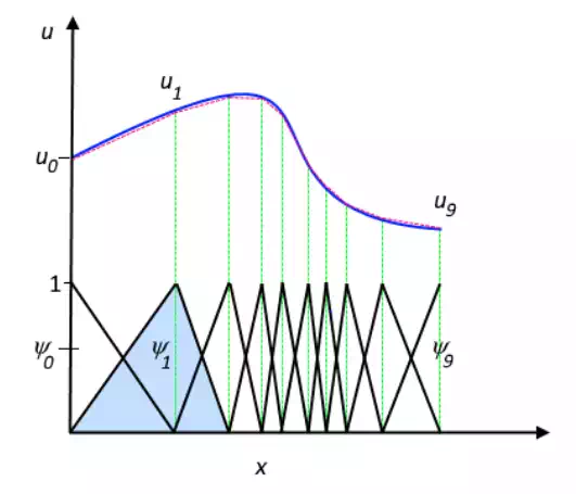
The function u (solid blue line) is approximated with u_h (dashed red line), which is a linear combination of linear basis functions (ψ_i is represented by the solid black lines). The coefficients are denoted by u₀ through u₇. Both of these figures show that the selected linear basis functions include very limited support (nonzero only over a narrow interval) and overlap along the x-axis. Depending on the problem at hand, other functions may be chosen instead of linear functions.

Another benefit of the finite element method is that the theory is well developed. The reason for this is the close relationship between the numerical formulation and the weak formulation of the PDE problem (see the section below). For instance, the theory provides useful error estimates, or bounds for the error, when the numerical model equations are solved on a computer. Looking back at the history of FEM, the usefulness of the method was first recognized at the start of the 1940s by Richard Courant, a German-American mathematician. While Courant recognized its application to a range of problems, it took several decades before the approach was applied generally in fields outside of structural mechanics, becoming what it is today.

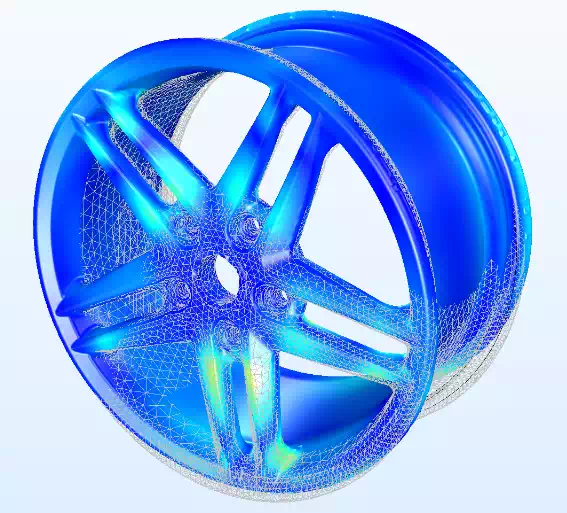
Finite element discretization, stresses, and deformations of a wheel rim in a structural analysis.

Algebraic Equations, Ordinary Differential Equations, Partial Differential Equations, and the Laws of Physics The laws of physics are often expressed in the language of mathematics. For example, conservation laws such as the law of conservation of energy, conservation of mass, and conservation of momentum can all be expressed as partial differential equations(PDEs). Constitutive relations may also be used to express these laws in terms of variables like temperature, density, velocity, electric potential, and other dependent variables. Differential equations include expressions that determine a small change in a dependent variable with respect to a change in an independent variable (x, y, z, t). This small change is also referred to as the derivative of the dependent variable with respect to the independent variable.

Say there is a solid with time-varying temperature but negligible variations in space. In this case, the equation for conservation of internal (thermal) energy may result in an equation for the change of temperature, with a very small change in time, due to a heat source g:

Here,  denotes the density and C_p denotes the heat capacity. Temperature, T, is the dependent variable and time, t, is the independent variable. The function  may describe a heat source that varies with temperature and time. Eq. (3) states that if there is a change in temperature in time, then this has to be balanced (or caused) by the heat source . The equation is a differential equation expressed in terms of the derivatives of one independent variable (t). Such differential equations are known as ordinary differential equations (ODEs).

In some situations, knowing the temperature at a time t₀, called an initial condition, allows for an analytical solution of Eq. (3) that is expressed as:

The temperature in the solid is therefore expressed through an algebraic equation (4), where giving a value of time, t₁, returns the value of the temperature, T₁, at that time.

Oftentimes, there are variations in time and space. The temperature in the solid at the positions closer to a heat source may, for instance, be slightly higher than elsewhere. Such variations further give rise to a heat flux between the different parts within the solid. In such cases, the conservation of energy can result in a heat transfer equation that expresses the changes in both time and spatial variables (x), such as:

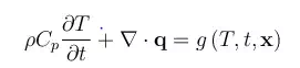
As before, T is the dependent variable, while x (x = (x, y, z)) and t are the independent variables. The heat flux vector in the solid is denoted by q = (q_x, q_y, q_z) while the divergence of q describes the change in heat flux along the spatial coordinates. For a Cartesian coordinate system, the divergence of q is defined as:

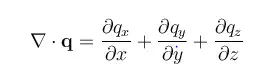
Eq. (5) thus states that if there is a change in net flux when changes are added in all directions so that the divergence (sum of the changes) of q is not zero, then this has to be balanced (or caused) by a heat source and/or a change in temperature in time (accumulation of thermal energy).

The heat flux in a solid can be described by the constitutive relation for heat flux by conduction, also referred to as Fourier’s law:

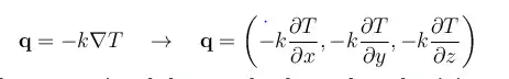
In the above equation, k denotes the thermal conductivity. Eq. (7) states that the heat flux is proportional to the gradient in temperature, with the thermal conductivity as proportionality constant. Eq. (7) in (5) gives the following differential equation:

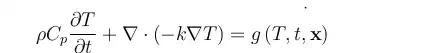
Here, the derivatives are expressed in terms of t, x, y, and z. When a differential equation is expressed in terms of the derivatives of more than one independent variable, it is referred to as a partial differential equation (PDE), since each derivative may represent a change in one direction out of several possible directions. Further note that the derivatives in ODEs are expressed using d, while partial derivatives are expressed using the more curly ∂.

In addition to Eq. (8), the temperature at a time t₀ and temperature or heat flux at some position x₀ could be known as well. Such knowledge can be applied in the initial condition and boundary conditions for Eq. (8). In many situations, PDEs cannot be resolved with analytical methods to give the value of the dependent variables at different times and positions. It may, for example, be very difficult or impossible to obtain an analytic expression such as:

from Eq. (8).

Rather than solving PDEs analytically, an alternative option is to search for approximate numerical solutions to solve the numerical model equations. The finite element method is exactly this type of method – a numerical method for the solution of PDEs.

Similar to the thermal energy conservation referenced above, it is possible to derive the equations for the conservation of momentum and mass that form the basis for fluid dynamics. Further, the equations for electromagnetic fields and fluxes can be derived for space- and time-dependent problems, forming systems of PDEs.

Continuing this discussion, let's see how the so-called weak formulation can be derived from the PDEs.