The finite difference method

The finite difference approximations for derivatives are one of the simplest and of the oldest methods to solve differential equations. It was already known by L. Euler (1707-1783) ca. 1768, in one dimension of space and was probably extended to dimension two by C. Runge (1856-1927) ca. 1908. The advent of finite difference techniques in numerical applications began in the early 1950s and their development was stimulated by the emergence of computers that offered a convenient framework for dealing with complex problems of science and technology. Theoretical results have been obtained during the last five decades regarding the accuracy, stability and convergence of the finite difference method for partial differential equations.

Finite difference approximations

General principle                                                                                   

The principle of finite difference methods is close to the numerical schemes used to solve ordinary differential equations (cf. Appendix C). It consists in approximating the differential operator by replacing the derivatives in the equation using differential quotients. The domain is partitioned in space and in time and approximations of the solution are computed at the space or time points. The error between the numerical solution and the exact solution is determined by the error that is commited by going from a differential operator to a difference operator. This error is called the discretization error or truncation error. The term truncation error reflects the fact that a finite part of a Taylor series is used in the approximation.

For the sake of simplicity, we shall consider the one-dimensional case only. The main concept behind any finite difference scheme is related to the definition of the derivative of a smooth function u at a point x ∈ R:

and to the fact that when h tends to 0 (without vanishing), the quotient on the right-hand side provides a ”good” approximation of the derivative. In other words, h should be sufficiently small to get a good approximation. It remains to indicate what exactly is a good approximation, in what sense. Actually, the approximation is good when the error commited in this approximation (i.e. when replacing the derivative by the differential quotient) tends towards zero when h tends to zero. If the function u is sufficiently smooth in the neighborhood of x, it is possible to quantify this error using a Taylor expansion.

Taylor series

Suppose the function u is C2 continuous in the neighborhood of x. For any h > 0 we have:

where h1 is a number between 0 and h (i.e. x + h1 is point of ]x, x + h[). For the treatment of problems, it is convenient to retain only the first two terms of the previous expression:

where the term O(h2) indicates that the error of the approximation is proportional to h2. From the equation (6.1), we deduce that there exists a constant C > 0, such that for h > 0 sufficienty small we have:

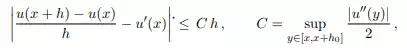
for h ≤ h0 (h0 > 0 given). The error commited by replacing the derivative u! (x) by the differential quotient is of order h. The approximation of u! at point x is said to be consistant at the first order. This approximation is known as the forward difference approximant of u! . More generally, we define an approximation at order p of the derivative.

A finite difference scheme

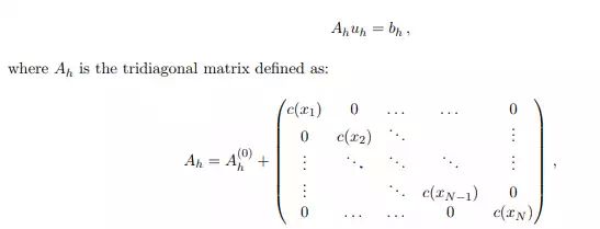
Suppose functions c and f are at least such that c ∈ C0(Ω¯) and f ∈ C0(Ω¯). The problem is then to find uh ∈ RN , such that ui ( u(xi), for all i ∈ {1, . . . , N}, where u is the solution of problem (6.3). Introducing the approximation of the second order derivative by a differential quotient, we consider the following discrete problem:

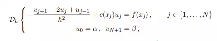
The problem D has been discretized by a finite difference method based on a three-points centered scheme for the second-order derivative. The problem (6.4) can be written in the matrix form as: