Special Cases in Nodal
Analysis
This article
describes certain special cases when performing nodal analysis.
When we are designing
electronic circuits, it is always important to know how much current is flowing
through a component or how much voltage is present at a particular node in the
circuit at crucial points in its operation. Finding either measurement can be
done using Kirchhoff’s circuit laws. The two analysis types that allow us to
find these values are Mesh Analysis and Nodal Analysis. If we are seeking to
find the voltage at a point (node), then we can apply nodal analysis using
Kirchhoff’s Current Law (KCL).
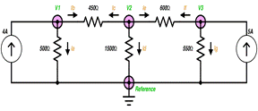
Each specific node in this
schematic (V1, V2, and V3) has 3 connections. KCL declares that the sum of all
branch currents from each node is zero. We can use this to find the voltage at
each node by the following method:
First, we have a reference
node with the lowest potential which will be called the ground. The ground in
this circuit is chosen because it is a common point with the lowest voltage.
Next, we assign a variable to each node where the voltage is unknown. This is
marked by the circles at V1, V2, and V3.Third, apply KCL to form an equation
for each unknown voltage.
For node V1:
The currents Ia and Ib:
IaIa
=
V1500ΩV1500Ω
and
Ib=(V1−V2)450ΩIb=(V1−V2)450Ω
It is because the voltage
thru the resistor is the difference of potential between its two nodes. Since
V1 is the only node directly connected to the 4 amp current source,
Ia+Ib=4AmpsIa+Ib=4Amps
.
Putting this all together:
V1500Ω+(V1−V2)450Ω=4AmpsV1500Ω+(V1−V2)450Ω=4Amps
.
This can be rewritten as:
V1(1500Ω+1450Ω)−V2(1450Ω)=4AmpsV1(1500Ω+1450Ω)−V2(1450Ω)=4Amps
.
For node V2:
Ic is pointing from V2 to V1 so we
will write the 450Ω resistor branch as:
(V2−V1)450Ω(V2−V1)450Ω
.
Id is simply:
V21500ΩV21500Ω
.
Ie flows from V2 to V3 and it is
noted as:
(V2−V3)600Ω(V2−V3)600Ω
.
Remember that KCL requires
the sum of all 3 branches to be zero. This means
Ic+Id+Ie=0Ic+Id+Ie=0
.
As one formula, it is put
together as:
(V2−V1)450Ω+V21500Ω+(V2−V3)600Ω=0(V2−V1)450Ω+V21500Ω+(V2−V3)600Ω=0
.
A friendlier form for linear
equations would be:
−V1(1450)+V2(1450+11500+1600)−V3(1600)=0−V1(1450)+V2(1450+11500+1600)−V3(1600)=0
.
Node V3 is the same
construction as node V1, only with different values.
Ig is:
V3550ΩV3550Ω
.
If (eye-eff, not iff. English mocks us!) is:
(V3−V2)600Ω(V3−V2)600Ω
.
Both resistors are fed from
the 5-Amp source, making
If+Ig=5AIf+Ig=5A
.
Put together, we have:
(V3−V2)600Ω+V3550Ω=5A(V3−V2)600Ω+V3550Ω=5A
.
Prettied up for calculation,
the equation is:
–V2(1600)+V3(1550+1600)=5–V2(1600)+V3(1550+1600)=5
.
The fourth and last step is
to solve the system of equations. There are calculators that can solve systems
of linear equations. Matlab and GNU Octave are
pc programs that can perform this function. With a pencil, paper, and 20
minutes of time; we could solve this “Old School” using Algebra. However we
might as well use a faster and possibly more reliable method, so let’s go with
an online option of www.wolframalpha.com.
Our three final equations can
be grouped together as:
v1(1500+1450−v2(1450)=4v1(1500+1450−v2(1450)=4
,
−v1(1450)+v2(1450+11500+1600)−v3(1600)=0−v1(1450)+v2(1450+11500+1600)−v3(1600)=0
,
–v2(1600)+v3(1550+1600)=5–v2(1600)+v3(1550+1600)=5
.
Though this is mathematically
correct, WolframAlpha basically replied
with “huh”?.
To make the formula a little
more agreeable, let’s throw in “*” for multiplication:
v1∗(1500+1450−v2∗(1450)=4v1∗(1500+1450−v2∗(1450)=4
,
−v1∗(1450)+v2∗(1450+11500+1600)−v3∗(1600)=0−v1∗(1450)+v2∗(1450+11500+1600)−v3∗(1600)=0
,
–v2∗(1600)+v3∗(1550+1600)=5–v2∗(1600)+v3∗(1550+1600)=5
.
The solution is a bit messy as
v1=31590001697−−−−−−−−−−−v1=31590001697_
.
But clicking approximate form
on the web page will yield:
v1=1,861.5−−−−−−−−−−v1=1,861.5_
,
v2=1,736.9−−−−−−−−−−v2=1,736.9_
and
v3=2,265.5−−−−−−−−−−v3=2,265.5_
.
To check this, compare power
flowing into the circuit from both sources to power being dissipated by the
resistors. The node V1 has 1,861.5 Volts with 4 Amps equaling 7,446
Watts. At 2,265.5 Volts @ 5 Amps, node V3 has 11,327.5 Watts. Resistors are
producing heat at the following rate: 450 Ω 34.5 Watts, 500 Ω
6,930.36 Watts, 1500 Ω 2,011.21 Watts, 600 Ω 465.7 Watts, and 550
Ω 9,331.8 Watts. Power in is 18,773.5 Watts. Power dissipated is 18,773.57
Watts due to rounding issues. Either we have designed the world’s most powerful
toaster oven, or our current should been a bit less for this example!
Special Cases: Voltage
Sources and Supernodes.
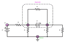
The addition of voltage
sources presents a special case situation. Here we have a 6 volt source and 3
volt source. The 3 volt source is between two non-reference nodes and forms
a supernode.
Finding the reference node is
same process as it was in the last example.
Now things change a little
bit. The 6V node does not require KCL because we already know the circuit is 6
volts at this location. The supernode is
not as bad as it looks, we just need to have a KVL equation added. The V2 side
of the 3 volt battery has a higher voltage potential than the V1 side, so the KVL
we will use is
V2−V1=3VV2−V1=3V
.
The KCL for the rest of the
circuit is:
(V1−6v)5Ω+V13Ω+V22Ω+V28Ω=0(V1−6v)5Ω+V13Ω+V22Ω+V28Ω=0
.
You may have noticed that the
math isn’t as messy in this example. We chose to divide by the resistance rather
than multiply by the reciprocal. Either way is perfectly valid.
Hey! What about the 4 Ω
resistor? No one wants to be left out! Well, the 4 Ω resistor is part of a
package deal. It is seen as part of the supernode and
does not have to be factored in as a separate equation. Lucky us!
We can add a few parentheses
to our linear equations to make things a bit more clear and input them into
the WolframAlpha page as:
v2−v1=3v2−v1=3
,
(v1−6)5+(v1)3+(v2)2+(v2)8=0(v1−6)5+(v1)3+(v2)2+(v2)8=0
.
Lo and behold, we find:
V1=−0.5827−−−−−−−−−−−V1=−0.5827_
and
V2=2.4173−−−−−−−−−−V2=2.4173_
as our answer.
As complex as this may seem,
nodal analysis is the basis for many circuit simulation programs and is a
cornerstone for understanding voltages at intersecting points in a circuit.