Analysis of Forward Conducting Diodes

In this article, we will learn how to analyze circuits that utilize forward conducting diodes. We will also talk about the exponential model, constant voltage drop model, as well as the ideal diode model.

Forward Characteristics of a Diode

Having read the previous article in this series, you should have an understanding of the diode terminal characteristics. From this previous knowledge, we will now delve into analyzing circuits that utilize forward conducting diodes. The figure below, Figure 1.1, illustrates a circuit that consists of a DC source, a resistor, as well as a diode. We will analyze this circuit and determine the diode’s current ID and voltage VD. For a better understanding, we will represent the diode with a model. 

The Exponential Model

A diode operating in the forward region can be most accurately described by the exponential model. However, due to it being extremely nonlinear, it is very difficult to use. Anyways, we will illustrate its accurate yet severe nonlinear behavior by analyzing the circuit shown in Figure 1.1.

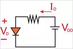
Figure 1.1 Simplistic circuit used for analyzing a forward-conducting diode.

Recall from the previous article that IS is a constant for a given diode at a given temperature. There is a formula that is used to calculate the value for IS, the reverse saturation current, in terms of the diode's temperature and parameters that we will not explain in this article.

When VDD is high enough to cause the diode’s forward current (ID) to be much larger than its saturation current, we can approximate the current–voltage relationship with the following exponential equation:

ID=ISeVD/nVTID=ISeVD/nVT

Equation 1.1

where VT is approximately 25 mV at room temperature and n is a constant influenced by the diode’s physical structure and fabrication process. For simplicity, in this article we will assume that n = 1.

This equation indicates that the forward current increases exponentially with respect to the forward voltage.

There is another equation that regulates how the circuit operates and is obtained by writing out a Kirchhoff loop, which results in 

ID=VDD−VDRID=VDD−VDR

Equation 1.2

Analyzing the Exponential Model Graphically

We will use Equations 1.1 and 1.2 by plotting their relationships and characteristics on a current vs. voltage plane. The intersection point of the two graphs plotted on the same axes is the solution, or the operating point Q. The two equations are illustrated in Figure 1.2.

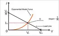
Figure 1.2 Plot of the circuit in Figure 1.1 as well as Equations 1.1 and 1.2

The curve that is plotted in Figure 1.2 represents the exponential diode equation, or Equation 1.1, and the straight line that slopes downwards represents Equation 1.2. This straight line is referred to what is known as the load line. This load line represents the constraint of other parts of the circuit place on a non-linear device (such as a diode or even a transistor). The exponential curve is the diode's characteristic curve. The operating point of the circuit has coordinates that give the values of ID and VD.

By analyzing the exponential diode model graphically, we can gain a better understanding visually how the circuit will work. However, to actually perform such an analysis is considered to be very tedious and requires much effort, especially for complex circuits. 

Analyzing the Exponential Model Iteratively

The solutions to Eqs 1.1 & 1.2 can be found through a rather straightforward iterative process, which is illustrated in the following example.

---

Example:

Analyze the circuit in Figure 1.1 with R = 2 kΩ and VDD = 5 V to determine the current ID as well as the diode's voltage VD. We can assume that the diode's current of 2 mA at a voltage of 0.7 V.

Solution:

With VD = 0.7 V and Equation 1.2, the current can be found as follows:

ID=VDD−VDRID=VDD−VDR

=5V−0.7V2kΩ=2.15mA=5V−0.7V2kΩ=2.15mA

By applying the equation illustrated in the previous article, we can obtain a more accurate value for VD. 

V2−V1=2.3VTlogI2I1V2−V1=2.3VTlogI2I1

If we assume that 2.3VT = 60 mV, we have

V2=V1+0.06V⋅logI2I1V2=V1+0.06V⋅logI2I1

Using the diode's voltage and current as V1 = 0.7 V and I1 = 2 mA, as well as I2 = 2.15 mA provides a value of V2 = 0.70188 V. The values from the first iteration are ID = 2.15 mA and VD = 0.70188 V. Iterating a second time provides the following values:

ID=5V−0.70188V2kΩ=2.149mAID=5V−0.70188V2kΩ=2.149mA

V2=0.70188V+0.06log[2.149mA2.15mA]V2=0.70188V+0.06log[2.149mA2.15mA]

=0.70187V=0.70187V

This second iteration provides values of  ID = 2.149 mA and VD = 0.70187 V. Since the second iteration provided values that are extremely close to those of the first iteration, the iteration process is complete. Thus the solution is ID = 2.149 mA and VD = 0.70187 V.

Constant-Voltage-Drop Model

Of all the models, the simplest and most commonly used in modeling the diode is the constant-voltage-drop (CVD) model. The CVD model uses the fact that any forward conducting diode has a voltage drop that fluctuates in a rather narrow range (~ 0.6 to 0.8 V). In this model, we assume that the voltage is at a constant value of 0.7 V. This assumption is better explained in Figure 1.3.

The CVD model is perhaps one of the most often utilized in the beginning stages of analysis and design of any circuitry. Also, at any point, if there is little to no information detailing the diode’s characteristics, this model is used quite frequently as well.

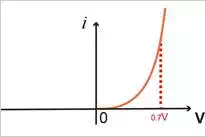
Figure1.3 (A) The exponential characteristic of the diode

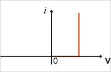
Figure 1.3 (B) Approximation of the exponential characteristic of the diode from a constant voltage value (usually assumed to be 0.7 V)

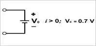
Figure 1.3 (C) The CVD model of a forward conducting diode

Lastly, if we apply the CVD model to solve our previous example, we are provided with

VD = 0.7 V

thus,

ID=VDD−0.7VRID=VDD−0.7VR

=5V−0.7V2kΩ=2.15mA=5V−0.7V2kΩ=2.15mA

which isn't too far off from the values previously obtained with a more extensive, exponential model.

Ideal Diode Model

In many instances, applications that involve voltage values that are much greater than that used in the CVD model (0.6 - 0.8 V), neglect the diode's voltage drop completely whilst computing the diode current. This is what is known as the ideal diode model. For the circuit that was used in the previous example with its values, we see that applying this model provides us with 

VD=0VVD=0V

ID=5V−0V2kΩ=2.5mAID=5V−0V2kΩ=2.5mA

For an analysis this quick, such an answer would not be an entirely bad estimate. However, the 0.7 V CVD model provides a much more accurate result almost no more work needed to be done. This model is great for determining which diodes are on or are off in a circuit containing multiple diodes.

Conclusion

In this article, we discussed the characteristics of forward conducting diodes, the exponential model, the CVD model, as well as the ideal diode model. As of now, you should have an understanding of each model, what its applications are, as well as be able to solve problems using each model. 

In the next article, we will build off of this article and talk about the small signal model and how the diode forward drop is used in voltage regulation.

Thank you for reading. If you have any questions or comments, please leave them below!