Norton Theorem
This theorem is just alternative of Thevenin theorem.
In Norton theorem, we just replace the circuit connected to a
particular branch by equivalent current source. In this theorem, the circuit network is
reduced into a single constant current source in which, the equivalent internal resistance is
connected in parallel with it. Every voltage source can be converted into equivalent current
source.
Suppose, in complex network we have to find out the current through
a particular branch. If the network has one of more active sources, then it
will supply current through the said branch. As in the said
branch current comes from the network, it can be considered that the network
itself is a current source. So in Norton theorem the network
with different active sources is reduced to single current
source that's internal resistance is nothing but the looking back
resistance, connected in parallel to the derived source.
The looking back resistance of a network is the equivalent electrical
resistance of the network when someone looks back into the network
from the terminals where said branch is connected. During calculating this
equivalent resistance, all sources are removed leaving their internal
resistances in the network. Actually in Norton theorem, the branch of the
network through which we have to find out the current, is
removed from the network. After removing the branch, we short circuit the
terminals where the said branch was connected. Then we calculate the short
circuit current that flows between the terminals. This current is nothing but Norton
equivalent current IN of the source. The equivalent resistance between
the said terminals with all sources removed leaving their internal resistances
in the circuit is calculated and said it is RN. Now we will form a current
source that's current is IN A and internal
shunt resistance is RN Ω.
For getting clearer concept of this theorem, we have explained it by the
following example,
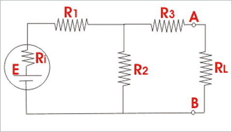
In the example two resistors R1 and R2 are
connected in series and this series combination is connected across one voltage
source of emf E with
internal resistance Ri as shown.
Series combination of one resistive branch of RL and another
resistance R3 is connected across the resistance R2 as
shown. Now we have to find out the current through RL by applying
Norton theorem.
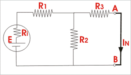
First, we have to remove the resistor RL from terminals A and B
and make the terminals A and B short circuited by zero resistance.
Second, we have to calculate the short circuit current or Norton
equivalent current IN through the points A
and B.
The equivalent resistance of the network,
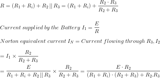
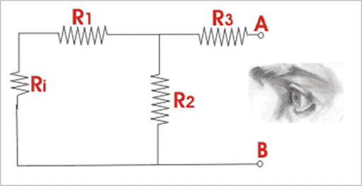
To determine internal resistance or Norton equivalent resistance RN of
the network under consideration, remove the branch between A and B and also
replace the voltage source by its internal resistance. Now the
equivalent resistance as viewed from open terminals A and B is RN,
![]()
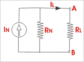
As per Norton theorem, when resistance RL is reconnected across
terminals A and B, the network behaves as a source of constant current IN with
shunt connected internal resistance RN and this is Norton
equivalent circuit.
Biot Savart Law
The mathematical expression for magnetic flux density was derived by Jean
Baptiste Biot and Felix Savart. Talking the
deflection of a compass needle as a measure of the intensity of a
current, varying in magnitude and shape, the two scientists concluded that any current element
projects into space a magnetic field, the magnetic flux density of which dB, is
directly proportional to the length of the element dl, the current I, the sine
of the angle and θ between direction of the current and the vector joining
a given point of the field and the current element and is inversely
proportional to the square of the distance of the given point from the current
element, r. This is Biot Savart
lawstatement. ![]()
Where, K is a constant, depends upon the magnetic properties of the medium and
system of the units employed. In SI system of unit,
![]()
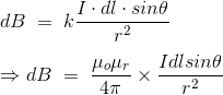
Therefore, final Biot Savart law derivation
is,
![]()
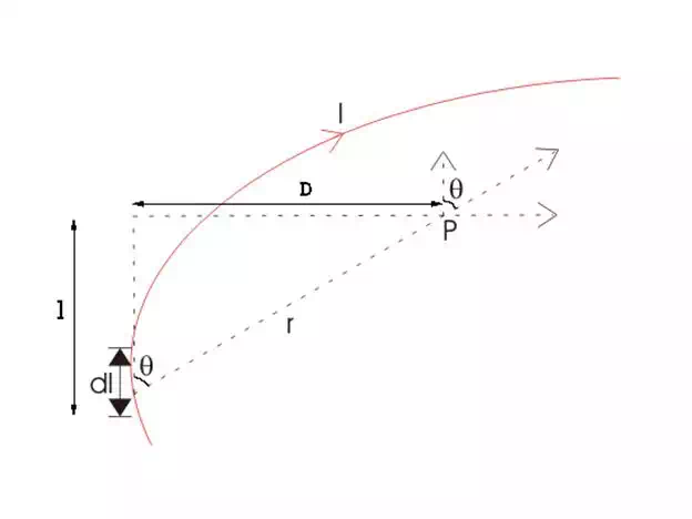
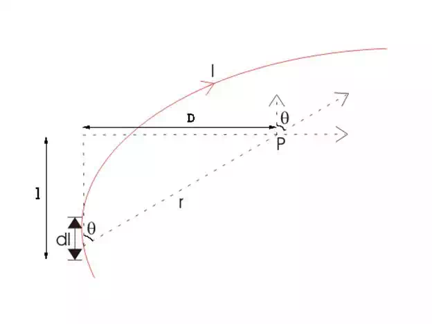
Let us consider a long wire carrying an current I and also consider a point p.
The wire is presented in the below picture by red color.
Let us also consider an infinitely small length of the wire dl at a distance r
from the point P as shown. Here, r is a distance vector which makes an angle
θ with the direction of current in the infinitesimal portion of the wire.
If you try to visualize the condition, you can easily understand the
magnetic field density at that point P due to that infinitesimal length dl of
wire is directly proportional to current carried by this portion of the wire.
That means current through this infinitesimal portion of the wire is increased
the magnetic field density due to
this infinitesimal length of wire, at point P increases proportionally and if the
current through this portion of wire is decreased the magnetic field density at
point P due to this infinitesimal length of wire decreases proportionally.
As the current through that infinitesimal length of wire is same as the current
carried by the wire itself.
![]()
It is also very natural to think that the magnetic field density at that point
P due to that infinitesimal length dl of wire is inversely proportional to the
square of the straight distance from point P to center of
dl. That means distance r of this infinitesimal portion of the wire is
increased the magnetic field density due to
this infinitesimal length of wire, at point P decreases and if the distance of
this portion of wire from point P, is decreased, the magnetic field density at
point P due to this infinitesimal length of wire increases accordingly.
![]()
Lastly, field density at that point P due to that infinitesimal portion of wire
is also directly proportional to the actual length of the infinitesimal length
dl of wire. As θ be the angle between distance vector r and direction of
current through this infinitesimal portion of the wire. The component of dl
directly facing perpendicular to the point P is dlsinθ,
![]()
Now combining these three statements, we can write,
![]()
This is the basic form of Biot Savart's Law
Now putting the value of constant k (which we have already introduced at the
beginning of this article) in the above expression, we get
Here, μ0 used in the expression of constant k is absolute
permeability of air or vacuum and it's value
is 4π10-7 Wb/ A-m in
SI system of units. μr of
the expression of constant k is relative permeability of the
medium.
Now, flux density(B) at the point P due to total length of the current carrying
conductor or wire can be represented as,
![]()
If D is the perpendicular distance of the point P form the wire, then
![]()
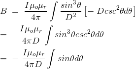
Now, the expression of flux density B at point P can be rewritten as,
![]()
![]()
As per the figure above,
![]()
Finally the expression of B comes as,
This angle θ depends upon the length of the wire and the position of the
point P. Say for certain limited length of the wire, angle θ as indicated
in the figure above varies from θ1 to θ2.
Hence, flux density at point P due to total length of the conductor is,
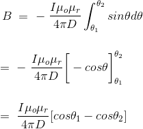
Let's imagine the wire is infinitely long, then θ will vary from 0 to
π that is θ1 = 0 to θ2 = π.
Putting these two values in the above final expression of Biot Savart law, we get,
![]()
This is nothing but the expression of Ampere's Law.