Transmission Lines: From Lumped Element to Distributed Element Regimes

Delving further into the transmission line concept, the boundary between treating the line as a single lumped circuit element and using the distributed circuit parameters is investigated with a simple analysis in python. Circuit parameters for multiple waveguide geometries are shown.

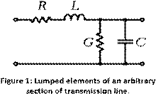
In the previous article Intro to the Long Transmission Line, the nature of the line parameters were derived from assuming that they could be considered distributed along the length of the line. The elements were modeled with series inductance per unit length

z=R+jωLz=R+jωL

and shunt admittance per unit length     

y=G+jωCy=G+jωC

. These are combined into the lumped section of transmission line

As discussed previously, at a certain length a wire must be considered for the effects it has on the overall system as a circuit element. Until the wire approaches such a length, it can be approximated as a singular lumped element whose values depend on the geometry of the waveguide and the medium it is made of. For an arbitrary geometry, the values for R, L ,C, and G can be derived given a few assumptions we will take for granted. Using the arbitrary waveguide profile in Figure 2 with transverse electric-magnetic waves (TEM) and fields

E¯E¯

and

H¯H¯

 , with cross sectional surface area S.

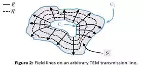
The voltage between conductors

C1C1

and

C2C2

are assumed to be

V0e±jβzV0e±jβz

and the current is of the form

I0e±jβzI0e±jβz

. The time averaged stored magnetic energy for a 1 meter section is

Wm=μ4∫SH¯⋅H¯∗dsWm=μ4∫SH¯⋅H¯∗ds

Circuit theory shows

Wm=L⋅|I0|2/4Wm=L⋅|I0|2/4

in terms of the current on the line. Thus self-inductance per unit length is

L=μ|I0|2∫SH¯⋅H¯∗dsH/mL=μ|I0|2∫SH¯⋅H¯∗dsH/m

Similarly, the time averaged electric energy per unit length is

We=ϵ4∫SE¯⋅E¯∗dsWe=ϵ4∫SE¯⋅E¯∗ds

Once again, circuit theory provides the relation

We=C⋅|V0|2/4We=C⋅|V0|2/4

which then gives the capacitance per unit length

C=ϵ|V0|2∫SE¯⋅E¯∗dsF/mC=ϵ|V0|2∫SE¯⋅E¯∗dsF/m

The power loss per unit length due to finite conductivity of the metallic conductors is given by the equation

PC=RS2∫S∣∣J¯∣∣2dsPC=RS2∫S|J¯|2ds

Which for this arbitrary geometry becomes:

PC=RS2∫C1+C2H¯⋅H¯∗dlPC=RS2∫C1+C2H¯⋅H¯∗dl

This is due to the assumption that

H¯H¯

is tangential to S. Circuit theory gives

PC=R⋅|I0|2/2PC=R⋅|I0|2/2

so the series resistance per unit length becomes

R=RS|I0|2∫C1+C2H¯⋅H¯∗dlΩ/mR=RS|I0|2∫C1+C2H¯⋅H¯∗dlΩ/m

Where

RS=1σδSRS=1σδS

is the surface resistance of the conductors, and

C1+C2C1+C2

is the integration path over the conductor boundaries. Similarly the conductance per unit length is from the equation for time averaged power dissipation per unit length in a lossydielectric

Pd=ωϵ′′|V0|2∫SE¯⋅E¯∗dsPd=ωϵ″|V0|2∫SE¯⋅E¯∗ds

where

ϵ′′ϵ″

is the imaginary part of the complex dielectric constant

ϵ=ϵ′+jϵ′′ϵ=ϵ′+jϵ″

. Utilizing circuit theory

Pd=G⋅|V0|2/2Pd=G⋅|V0|2/2

, we are then able to write the shunt conductance per unit length as

G=ωϵ′′|V0|2∫SE¯⋅E¯∗dsS/mG=ωϵ″|V0|2∫SE¯⋅E¯∗dsS/m

These equations should give the transmission line parameters for arbitrary waveguide geometries given that they support TEM modes, are uniform along the z axis (axis of signal propagation), and the solution to the travelling wave is the solution to the telegraphers equation derived in the previous article.

Some common geometries of waveguide are coaxial, two-wire, and parallel plate. To save you the computations that were just introduced, their values for inductance, capacitance, resistance, and conductance are as follows:

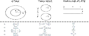
Where the complex permittivity constant

ϵ=ϵ′+jϵ′′ϵ=ϵ′+jϵ″

and permeability constant

μ=μ0μrμ=μ0μr

are unique to the materials used.

Given that we have the transmission line in terms of the circuit elements we are familiar with, why not just treat the entire line as the classification of the regions where the approximation of the transmission line as a single lumped element works accurately is referred to as short and medium length transmission lines. This is just to contrast when the model used must be the distributed element model when the transmission line is considered long.

To illustrate the difference between the regimes of analytical treatment of the transmission line, the different models are compared in a simulation for increasing lengths of line. From short-lines into the long-line regime, the analysis shows behavior of the load voltage (VL) using lumped and distributed element calculations for a lossless transmission line (where R=G=0). The frequency dependence is shown in the form of the line length being a multiple of wavelength.

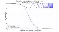
Depending on circuit sensitivity, the distributed model for transmission lines starts deviating from the simplified lumped element model between line length of 0.01x and 0.1x the wavelength of the signal. This simulation uses a load impedance that is close to the impedance of the transmission line, so the reflections are relatively small.

The specific threshold for relfection tolerance is determined by the application. Long transmission lines for utility power transmission can have a lower tolerance due to the large amounts of power being transmitted, so even small reflections can be of the magnitude of hundreds of kilowatts. In integrated circuits, small sensitive transistors operating at very high frequencies will have extremely small tolerances for power fluctuations, so again the threshold will be lower than in other applications.

# -*- coding: utf-8 -*-
"""
Created on Thurs Nov 19 17:18:24 2015

@author: Arthur
"""
import numpy as np
import math
import matplotlib.pyplot as plt

# Wire Model
# When does wire need to be treated as T-Line? And when
# does T-Line behavior deviate from simple lumped element?


def tanOfArray(some_array):
    c = np.array([np.tan(2*math.pi*a) for a in some_array])
return c

def expOfArray(some_array,sign):
    c = np.array([np.exp(sign*2j*math.pi*a) for a in some_array])
return c


# TL impedance
Zo = 50.0
# Source impedance
RS = 100.0
# Load impedance
RL = 100.0
# Source amplitude
Vs = 2.0
# Automatically generate title string for values above
title = "Distributed vs Lumped Element treatment of T-Line\n$R_S $ = "+str(int(RS))+" $\Omega $, "+"$R_L $ = "+str(int(RL))+" $\Omega $, "+"$Z_0 $ = "+str(int(Zo))+" $\Omega $"

# step (resolution) of inputs
SCALE = 0.001
# generate inputs
d = np.arange(0.001,10+SCALE,SCALE)

# Transmission line calculations
GL = (RL-Zo) / (RL+Zo)
num = RL + 1j*Zo*tanOfArray(d)
den = Zo + 1j*RL*tanOfArray(d)
Zin = Zo*(num / den)
Vin = Vs*Zin / (Zin+RS)
Vop = Vin / (expOfArray(d,1) + GL * expOfArray(d,-1))
vLTL = Vop*(1.0+GL) 
VLTL = np.abs(vLTL) #V_Load_Transmission_Line
phLTL = 180.0 * np.angle(vLTL) / math.pi #phase_Load_Transmission_line

#Lumped element calculations
A = -1j*Zo/(2*math.pi*d)
Z1 = (RL*A) / (RL + A)
Z2 = RS+2j*math.pi*Zo*d
vLle = Vs * Z1 / (Z1+Z2)
VLle = np.abs(vLle) # V_Load_lumped_element
phle = 180 * np.angle(vLle) / math.pi #phase_load_lumped_element

#generate plot
fig = plt.figure()
fig.suptitle(title, fontsize=30)
#ax1 = fig.add_subplot(211) #used if also plotting the phase in 2nd sublot
ax1 = fig.add_subplot(111)
plt.semilogx(d,VLTL,d,VLle,'--k', lw=3)
plt.ylabel('$V_L $ magnitude',fontsize=28)
plt.grid(True)
plt.legend(['T-Line model','Lumped Element model'],loc=3,fontsize=22)
ax1.tick_params(axis='x', labelsize=20)
ax1.tick_params(axis='y', labelsize=20)

"""
# ==================== 2nd plot unused this time ===============
# generate second plot for phase
ax2 = fig.add_subplot(212)
plt.semilogx(d,phLTL,d,phle,'--k',lw=2)
plt.axis([.01,10,-180,180])
g = plt.gca()
g.set_yticks(range(-180,181,60))
plt.ylabel('VL phase (deg)',fontsize=24)
plt.legend(['T-line model', 'lumped element model'],loc=3,fontsize=18)
plt.xlabel('Wire length - d (in multiples of wavelength)',fontsize=28)
plt.grid(True)
ax2.tick_params(axis='x', labelsize=18)
ax2.tick_params(axis='y', labelsize=18)
"""
plt.xlabel('Wire length - d (in multiples of wavelength)',fontsize=28)
plt.show()