Introduction to the Transmission Line

What's a transmission line and why does it exist? Find out!

When the physical dimension of a circuit approaches the magnitude of a wavelength of the signal, wires and circuit traces begin to affect circuit performance. This is due to the effects being frequency dependent and typically having very small values that are linearly dependent on wire/trace length. When the frequency and lengths become comparably large, the impedance becomes non-negligible. The ratio of wavelength to wire length can be considered as low as 0.01.

As a mental shortcut, so as not having to analyze the harmonic components of a signal, compare the rise time of the signal to the propagation delay. If the rise time is less than twice the propagation delay, transmission line effects must be considered. So if the propagation delay of a wire or trace is 5ns, then any signal with a rise time of less than 10ns will be affected due to transmission line effects.

To quantify this analytically, consider the familiar passive parasitics affecting a circuit’s performance: inductance, capacitance, resistance, and conductance (L, C, R, G). These elements can be thought of as being distributed along the length of the transmission line. For initial simplicity, the model is two parallel lines with 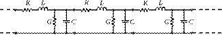one conductor and one ground.

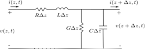
Examining a section of the lumped element model as a single mesh with Kirchoff’s voltage law, and using circuit elements whose values are per-unit length:

We get the equation:

$Title: v(z,t)-R\cdot \Delta z\cdot i(z,t)-L\cdot \Delta z\cdot \frac{\partial i(z,t)}{\partial t}-v(z+\Delta z,t)=0\; \; \; \; \; \; \;(eq. 1)$

Another analysis of the lumped element model with Kirchoff’s current law with one node at the top, gives the equation:

$Title: i(z,t)-G\cdot \Delta z\cdot v(z+\Delta z,t)-C\cdot \Delta z\cdot \frac{\partial v(z+\Delta z,t)}{\partial t}-i(z+\Delta z,t)=0\; \; \; \; \; \; \;(eq. 2)$

Divide both sides by

ΔzΔz

and take the limit as

Δz→0Δz→0

(note that the last terms become derivatives).

$Title: -R\cdot i(z,t)-L\cdot \frac{\partial i(z,t)}{\partial t}-\frac{\partial v(z,t)}{\partial z}=0\; \; \; \; \; \; \;(eq.\; 3)$

$Title: -G\cdot v(z,t)-C\cdot \frac{\partial v(z,t)}{\partial t}-\frac{\partial i(z,t)}{\partial z}=0\; \; \; \; \; \; \;(eq.\; 4)$

Simplify equations 3 and 4 using Cosine phasors.

$Title: \frac{\mathrm{d} V(z)}{\mathrm{d} z}=-(R+j\omega L)\cdot I(z)\; \; \; \; \; \; \;(eq.\; 5)$

$Title: \frac{\mathrm{d} I(z)}{\mathrm{d} z}=-(G+j\omega C)\cdot V(z)\; \; \; \; \; \; \;(eq.\; 6)$

We can then solve these equations simultaneously to find I(z) and V(z).

$Title: \frac{\mathrm{d^2} V(z)}{\mathrm{d} z^2}-\gamma^2\cdot I(z)=0\; \; \; \; \; \; \;(eq.\; 7)$

$Title: \frac{\mathrm{d^2} I(z)}{\mathrm{d} z^2}-\gamma^2\cdot V(z)=0\; \; \; \; \; \; \;(eq.\; 8)$

Equations 7 and 8 are commonly known as the telegraph equations. Where the

γγ

is the complex propagation constant:

$Title: \gamma =\sqrt{(R+j\omega L)(G+j\omega C)}\; \; \; \; \; \; \;(eq.\; 9)$

is for a single line and is a function of frequency.

Solving equations 7 & 8 for I(z) and V(z) give

$Title: V(z)=V_0^+\cdot e^{-\gamma z}+V_0^-\cdot e^{\gamma z}\; \; \; \; \; \; \;(eq.\; 10)$

$Title: I(z)=I_0^+\cdot e^{-\gamma z}+I_0^-\cdot e^{\gamma z}\; \; \; \; \; \; \;(eq.\; 11)$

Where

e−ωze−ωz

accounts for propagation in the positive z direction and

eωzeωz

for the reflection in the negative direction. If eq. 10 is plugged into eq. 8, we can get the relationship

$Title: I(z)=\frac{\gamma}{R+j\omega L}(V_0^+\cdot e^{-\gamma z}-V_0^-\cdot e^{\gamma z})\; \; \; \; \; \; \;(eq.\; 12)$

Comparing the terms in eq. 12 with eq. 11 leads to the conclusion that

$Title: \frac{V_0^+}{I_0^+}=Z_0=\frac{-V_0^-}{I_0^-}\; \; \; \; \; \; \;(eq. 13)$

In which case

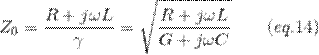
$Title: Z_0=\frac{R+j\omega L}{\gamma}=\sqrt{\frac{R+j\omega L}{G+j\omega C}}\; \; \; \; \; \; \;(eq. 14)$

and is defined as the characteristic impedance of the transmission line.

Using the characteristic impedance, we can define the current in terms of the voltage.

$Title: I(z)=\frac{V_0^+}{Z_0}\cdot e^{-\gamma z}-\frac{V_0^-}{Z_0}\cdot e^{\gamma z}\; \; \; \; \; \; \;(eq. 15)$

With the transmission line clearly defined as a circuit element, it can now be analyzed when a load is attached. We define the load to be located at z=0 to simplify the analysis.

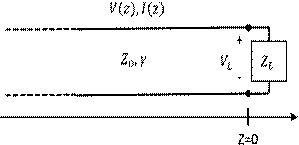
The current and voltage at the load can be related by the load impedence. Using equations 10 & 15, while setting z=0, we get

$Title: Z_L=\frac{V(0)}{I(0)}=\frac{V_0^++V_0^-}{V_0^+-V_0^-}\cdot Z_0 \; \; \; \; \; \; \;(eq. 16)$

Rearranging, we can find the reflected voltage value in terms of known values

$Title: V_0^-=\frac{Z_L-Z_0}{Z_L+Z_0}\cdot V_0^+\; \; \; \; \; \; \;(eq. 17)$

The ratio of reflected wave to the incident voltage wave is known as the reflection coefficient,

ΓΓ

$Title: \Gamma =\frac{V_0^-}{V_0^+}=\frac{Z_L-Z_0}{Z_L+Z_0}\; \; \; \; \; \; \;(eq. 18)$

An important case should be observed from eq. 18. When the load impedance matches the characteristic impedance of the transmission line, the reflection coefficient

Γ=0Γ=0

, and there is no reflected wave. This load is referred to as being matched to the transmission line.

Here is how the load matching effects the reflections in a transmission line.

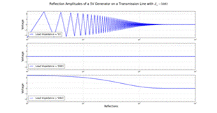
The first graph shows iterative reflections when the load is much smaller than

Z0Z0

, the second shows a load-matched transmission line with no reflections, and the third shows the same transmission line with a load that is much greater than Z0.

There you have it-- the fast and dirty intro to the transmission line!