Compound Interest Formulas
| An important concept throughout this course is the cash flow. The cash flow shows a collection of receipts and expenditures over time, and may be presented as a table or as a graph. Usually receipts are positive numbers with arrows pointing up on the graph, while disbursements are negative numbers with arrows pointing down. There will be cases when costs are the most important. Then we define disbursements as positive with arrows pointing up. Time is measured on the horizontal axis. For discrete compounding, time is measured in compounding periods. Although the compounding period is often one year, it may be some fraction of a year (one month, one quarter, one half). The numbers on the axis indicate compounding periods. In general the beginning and end points of the time range are arbitrary. The length of the range is N, and we assume that the start and end points are integer multiples of the compounding period. It is most common to have the range start at 0 and end at N. In the example on the left, N is 10.
|

Usually, we restrict cash flows to be located at integer time values. In practical problems, operating costs and revenues occur continuously, but for analysis, we collect all cash flows during a period and show them at the end of the period. This is called the end-of-the-period assumption. For example, the cash flows for the first period are shown at time 1. Major receipts or disbursements are shown where they occur, but only at integer values of time. The example has an investment at time 0.
Dollar values are measured by the vertical axis. These values may be scaled to accommodate large amounts.
On this page we consider simple patterns of cash flow. In the next lesson we show how more complicated cash flows like the one above can be represented by a collection of simple patterns.
We recognize four patterns of cash flow in terms of their location in time: present worth, future worth, uniform series and arithmetic gradient series.
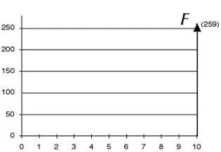
P: Present Worth This is the present worth (or present value). Without a subscript it is a single amount at time 0, where time 0 usually represents the present. |
|
F: Future Worth This is the future worth of a cash flow. Without a subscript, it is a single value at the end of the interval. |
|
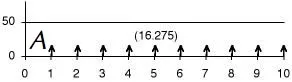
A: Uniform Series This is a series of equal cash flows over a given interval. The individual cash flows occur at the end of each period in the interval. This is the end-of-the-period assumption. The series name is based on the first letter of annuity. An annuity is a series of annual payments, but we allow the series to be defined for any compounding period. |
|
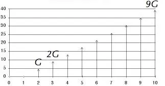
G: Gradient This is the step in values for a series of arithmetically increasing cash flows. The value of the cash flow at time t is G(t-1). For time 1 the cash flow is 0, for time 2, the cash flow is G, for time 3, the cash flow is 2G, and so on until for time N the cash flow is (N-1)G. It is important to note that the first term of a gradient series is always zero. |
|
| We use subscripts to refer to a single cash flow at time t. When working with an interval, such as 0-10 for these examples, the value of t need not be in the interval. For example |

| Equivalence Factors |
Ø For most of our applications, it will be necessary to move the components of a cash flow so that the result is a single value or a uniform series over a given interval. This is done using equivalence factors. Each factor changes one cash flow pattern to an equivalent pattern.
Ø To understand how the factors are used, a set of questions is given in the window called Simple Time Value. To perform the time value of money calculations, we can use the Factor Calculator, which resides in the Toolbox in the Computation Directory, or the factor tables discussed below.
Ø To begin, click the Q icon to open the questions.